IRIS-Dataset-Classification-using-ANN

Classify the IRIS Dataset using ANN from scratch.

Introduction

The IRIS dataset contains 150 samples in 3 different classes named "Setosa", "Versicolor", and "Virginica". There are 4 factors which determine the class of each sample. The Factors are sepal length in cm, sepal width in cm, petal length in cm, and petal width in cm. For more Information and to download the dataset you can simply go to this LINK.

Importing libraries

Obviously, the first part of each project is to import necessary libraries and since this project is from scratch we only import 3 libraries.

import pandas as pd
import numpy as np
from matplotlib import pyplot as plt

Data preprocessing

To load the Data, you can download it from the link in the Introduction, then you can read the data using pandas library.

data = pd.read_csv("[file directory]")

To get a simple information about the data you can use data.head() and see what the data looks like.

print(data.head())

The output should be something like this.

	sepal.length	sepal.width	petal.length	petal.width	variety
0	5.1	3.5	1.4	0.2	Setosa
1	4.9	3.0	1.4	0.2	Setosa
2	4.7	3.2	1.3	0.2	Setosa
3	4.6	3.1	1.5	0.2	Setosa
4	5.0	3.6	1.4	0.2	Setosa

To work with the data you should convert it to array. To do that you can use numpy library.

data = np.array(data)

In order to have a fair training set, use random.shuffle().

np.random.shuffle(data)

Note that data = np.random.shuffle(data) does not work.

At this point, we are ready to start splitting the data into training and test set. It is optional but in general, putting 80% of the data in the training data set is the optimum ratio. In this case, we have 120 samples in training set and 30 samples in the testing set. Do not forget to reshape() them to avoid furthere errors.

data_train = data[:-30].T
x_train = data_train[:-1]
x_train = x_train.reshape(120, 4)
y_train = data_train[-1]
y_train = y_train.reshape(120, 1)

data_test = data[-30:].T
x_test = data_test[:-1]
x_test = x_test.reshape(30, 4)
y_test = data_test[-1]
y_test = y_test.reshape(30, 1)

Building ANN

Intro

This section has 3 main parts. The first part is feeding the input data to the network and then calculate the output. The second part is calculating the backward propagation in order to calculate the error with respect to each weight. Last but not least, updating the weights.

In this project I am using the simplest ANN which has 2 layers, one hidden layer with 10 neurons and one output layer.

After each section, each variable will be defined.

Initializing the weight

For each layer we need to set weight at random in the range of [-0.5, 0.5]. To do this, we need to use np.random.rand().

vij = np.random.rand(10, 4) - 0.5
v0j = np.random.rand(10, 1) - 0.5
wjk = np.random.rand(3, 10) - 0.5
w0k = np.random.rand(3, 1) - 0.5

• vij matrix is the weights for the hidden layer.
• v0j matrix is the bias for the hidden layer.
• wjk matrix is the weights for the output layer.
• wjk matrix is the bias for the output layer.

• Note that we need to subtract each number from 0.5 to generate the weights in range of [-0.5, 0.5]. The Dimensions are set with respect to the input data and the number of neurons in the hidden layer and the output layer.

Forward propagation

The first thing we need to do is to feed the training set to the network with matrix multiplication.

z_inj = np.dot(vij, xi).reshape(10, 1) + v0j

• z_inj matrix is the input value of first hidden layer.
• xi matrix is the input data in shape of (4, 1)

Next, we need to activate the value of the hidden layer. There are many activation funcations that you can use but the common one is ReLU. This activation function is simple and is used for simple activating to reduce the calculating time. The function is indicated in the graph below.

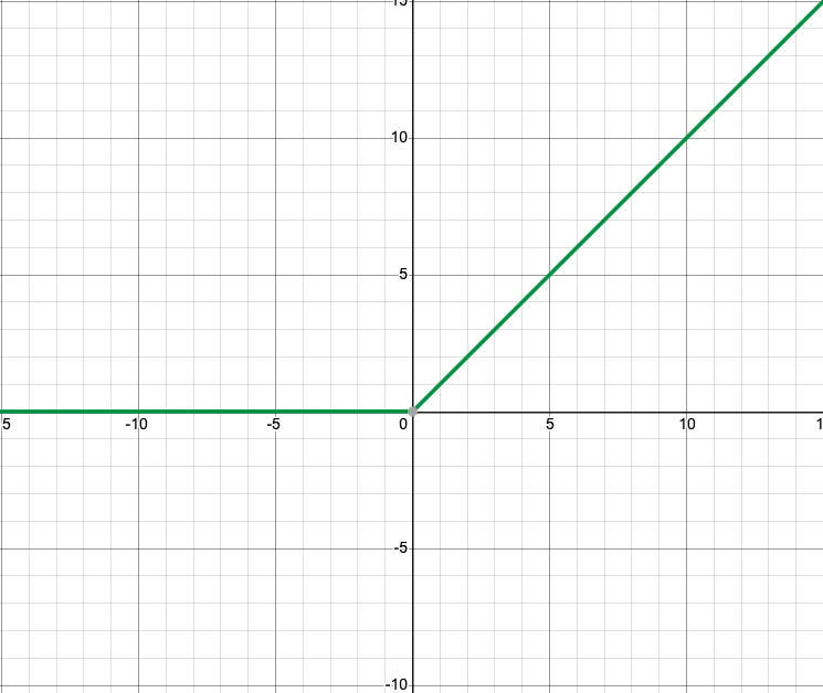
As you can see, It returns the value itself when the value is more than zero, and it returns the zero when the value is less then zero.

def relu(x):
    return np.maximum(0, x)

zj = relu(z_inj)

• zj matrix is the activated value of the hidden layer.

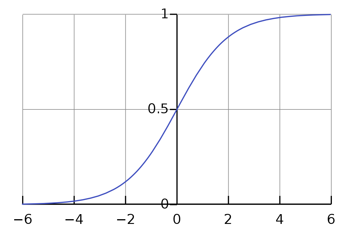
The next step is to do the same for the output layer but this time we use zj as input for the ouput layer alternatively. The activation function for the output layer is Sigmoid. This function allows us to calculate the probability of each class and in addition to that, its derivetive is calculated by the function itself, that is used in backward propagration section.

def sigmoid(x):
    x = 1 / (1 + np.exp(x))
    return x

y_ink = np.dot(wjk, zj).reshape(3, 1) + w0k
yk = sigmoid(y_ink)

• y_ink matrix is the input value of the output layer.
• yk matrix is the activated value of the output layer. (Predicted output)

Backward propagation

In this section, we need to calculate the error value of each layer. To do this, we need to use the derivative of the activation functions and some mathematics.

The cost function of the output layer is:

fpy_ink = sigmoid(y_ink) * (1 - sigmoid(y_ink))
dk = (yk - tk) * fpy_ink
dwjk = learning_rate * (np.dot(dk, zj.T))
dw0k = learning_rate * dk

• fpy_ink matrix is the derivative function of the sigmoid function.
• dk is a (n, 1) dimensional matrix that is used to calculate the error value of the weights.
• tk is a (n, 1) dimensional matrix that represents the real class of the input data. (Not the predicted one)
• dwjk matrix is the error of the wjk matrix. d stands for delta!
• dw0k matrix is the error of the w0k matrix (bias).

_{Note that for dk, dwjk, and dw0k we use the normal multiplication (Not np.dot()). This is because we want to multiply the value of each row in the dk to the each row of the all collumns in the dwjk and dw0k matrix.}

The cost function of the hidden layer is:

def g(x):
    return x>0

d_inj = np.dot(wjk.T, dk)
dj = d_inj * g(z_inj)
dvij = learning_rate * (np.dot(dj, xi.reshape(4,1).T))
dv0j = learning_rate * dj

• d_inj is the matrix of the error of the input signal for the hidden layer with respect to the error of weights for the output layer.
• dj is a (n, 1) dimensional matrix that is used to calculate the error value of the weights
• g() is the function that returns the derivative of the ReLU function. (That is 1 for the values grater than zero, and 0 for the otherwise)
• dvij matrix is the error of the vij matrix.
• dv0j matrix is the error of the v0j matrix.

Updating the weights

Last part of each iteration, is to update the weights. To to this, we can simply add the delta matrixes to their weights.

wjk = wjk + dwjk
w0k = w0k + dw0k
vij = vij + dvij
v0j = dv0j + dv0j

This was the whole idea of one iteration. in order to optimize the weight we need to do more iterations. There are 3 factors that decide how many times we have to repeat the iteration.

1. Constant error: Reaching the point that the weights do not differ from the last ones.
2. Number of iterations: Do it for determined number of iteration.
3. Accuracy: Reaching the optimal accuracy.

To calculate the accuracy, we need to feed the test data (x_test) to the network with updated weights and compare the predicted output of the network to the real one (y_test).