
home ::
syllabus ::
timetable ::
groups ::
moodle(591,
791) ::
video tbd ::
© 2021
Cluster, sort the leaves by their value, discretize the data to find the difference between the best and worst cluster.
What to hand in: code that handles all the TODO items listed below.
TODO : Generate this output using auto93.csv (and your results may differm slightly, due to random number differences).
     1	|..  n=398 c=0.71
     2	|.. |..  n=199 c=0.53
     3	|.. |.. |..  n=99 c=0.42
     4	|.. |.. |.. |..  n=49 c=0.25
     5	|.. |.. |.. |.. |..  n=24 c=0.15
     6	|.. |.. |.. |.. |.. |..  n=12	   goals=[3264.0, 16.5, 20.0]
     7	|.. |.. |.. |.. |.. |..  n=12	   goals=[3139.0, 15.5, 20.0]
     8	|.. |.. |.. |.. |..  n=25 c=0.27
     9	|.. |.. |.. |.. |.. |..  n=12	   goals=[2472.0, 15.5, 20.0]
    10	|.. |.. |.. |.. |.. |..  n=13	   goals=[2401.0, 16.5, 20.0]
    11	|.. |.. |.. |..  n=50 c=0.31
    12	|.. |.. |.. |.. |..  n=25 c=0.19
    13	|.. |.. |.. |.. |.. |..  n=12	   goals=[3381.0, 18.2, 20.0]
    14	|.. |.. |.. |.. |.. |..  n=13	   goals=[3233.0, 17.6, 20.0]
    15	|.. |.. |.. |.. |..  n=25 c=0.38
    16	|.. |.. |.. |.. |.. |..  n=12	   goals=[3415.0, 15.8, 20.0]
    17	|.. |.. |.. |.. |.. |..  n=13	   goals=[3035.0, 16.7, 20.0]
    18	|.. |.. |..  n=100 c=0.35
    19	|.. |.. |.. |..  n=50 c=0.22
    20	|.. |.. |.. |.. |..  n=25 c=0.18
    21	|.. |.. |.. |.. |.. |..  n=12	   goals=[4140.0, 13.7, 20.0]
    22	|.. |.. |.. |.. |.. |..  n=13	   goals=[3840.0, 13.9, 20.0]
    23	|.. |.. |.. |.. |..  n=25 c=0.12
    24	|.. |.. |.. |.. |.. |..  n=12	   goals=[4380.0, 13.2, 10.0]
    25	|.. |.. |.. |.. |.. |..  n=13	   goals=[4082.0, 13.5, 10.0]
    26	|.. |.. |.. |..  n=50 c=0.25
    27	|.. |.. |.. |.. |..  n=25 c=0.14
    28	|.. |.. |.. |.. |.. |..  n=12	   goals=[4456.0, 13.0, 10.0]
    29	|.. |.. |.. |.. |.. |..  n=13	   goals=[3892.0, 12.5, 20.0]
    30	|.. |.. |.. |.. |..  n=25 c=0.19
    31	|.. |.. |.. |.. |.. |..  n=12	   goals=[4464.0, 12.0, 10.0]
    32	|.. |.. |.. |.. |.. |..  n=13	   goals=[4422.0, 11.0, 10.0]
    33	|.. |..  n=199 c=0.58
    34	|.. |.. |..  n=99 c=0.48
    35	|.. |.. |.. |..  n=49 c=0.16
    36	|.. |.. |.. |.. |..  n=24 c=0.08
    37	|.. |.. |.. |.. |.. |..  n=12	   goals=[2420.0, 15.0, 30.0]
    38	|.. |.. |.. |.. |.. |..  n=12	   goals=[1985.0, 16.9, 40.0]
    39	|.. |.. |.. |.. |..  n=25 c=0.27
    40	|.. |.. |.. |.. |.. |..  n=12	   goals=[2515.0, 14.7, 30.0]
    41	|.. |.. |.. |.. |.. |..  n=13	   goals=[2020.0, 18.2, 30.0]
    42	|.. |.. |.. |..  n=50 c=0.2
    43	|.. |.. |.. |.. |..  n=25 c=0.17
    44	|.. |.. |.. |.. |.. |..  n=12	   goals=[2164.0, 15.9, 30.0]
    45	|.. |.. |.. |.. |.. |..  n=13	   goals=[2670.0, 15.5, 30.0]
    46	|.. |.. |.. |.. |..  n=25 c=0.09
    47	|.. |.. |.. |.. |.. |..  n=12	   goals=[2490.0, 17.3, 30.0]
    48	|.. |.. |.. |.. |.. |..  n=13	   goals=[2635.0, 16.0, 30.0]
    49	|.. |.. |..  n=100 c=0.54
    50	|.. |.. |.. |..  n=50 c=0.5
    51	|.. |.. |.. |.. |..  n=25 c=0.25
    52	|.. |.. |.. |.. |.. |..  n=12	   goals=[2003.0, 17.5, 30.0]
    53	|.. |.. |.. |.. |.. |..  n=13	   goals=[2489.0, 15.5, 20.0]
    54	|.. |.. |.. |.. |..  n=25 c=0.46
    55	|.. |.. |.. |.. |.. |..  n=12	   goals=[2130.0, 17.5, 30.0]
    56	|.. |.. |.. |.. |.. |..  n=13	   goals=[2265.0, 15.5, 20.0]
    57	|.. |.. |.. |..  n=50 c=0.29
    58	|.. |.. |.. |.. |..  n=25 c=0.16
    59	|.. |.. |.. |.. |.. |..  n=12	   goals=[2694.0, 15.5, 20.0]
    60	|.. |.. |.. |.. |.. |..  n=13	   goals=[1963.0, 15.5, 30.0]
    61	|.. |.. |.. |.. |..  n=25 c=0.31
    62	|.. |.. |.. |.. |.. |..  n=12	   goals=[2950.0, 15.9, 30.0]
    63	|.. |.. |.. |.. |.. |..  n=13	   goals=[2130.0, 15.8, 40.0]
Shown above is a cluster tree (technically speaking, a "dendogram") that you generated from last time. Recall that at each level, you found distant points then seperated the data on the median distance between the points.
In this print out of the tree, for non-leaves, I show
n:the size of the rows and the distancec: the distance between the two distant points
Note that c,n decrease as I go down the tree (why?).
For the leaves, I also show the median performance scores (Lbs-, Acc+, Mpg+). In the above, where is the best and worst cluster?
TODO : print out this sort order for the leaf clusters (and your results may differ slightly, due to random number differences).
     1	#Lbs-,   Acc+, Mpg+
     2
     3	[1985.0, 16.9, 40.0] <== best
     4	[2130.0, 15.8, 40.0]
     5	[2020.0, 18.2, 30.0]
     6	[2003.0, 17.5, 30.0]
     7	[1963.0, 15.5, 30.0]
     8	[2130.0, 17.5, 30.0]
     9	[2164.0, 15.9, 30.0]
    10	[2490.0, 17.3, 30.0]
    11	[2420.0, 15.0, 30.0]
    12	[2635.0, 16.0, 30.0]
    13	[2670.0, 15.5, 30.0]
    14	[2515.0, 14.7, 30.0]
    15	[2950.0, 15.9, 30.0]
    16	[2265.0, 15.5, 20.0]
    17	[2401.0, 16.5, 20.0]
    18	[2472.0, 15.5, 20.0]
    19	[2489.0, 15.5, 20.0]
    20	[2694.0, 15.5, 20.0]
    21	[3035.0, 16.7, 20.0]
    22	[3233.0, 17.6, 20.0]
    23	[3381.0, 18.2, 20.0]
    24	[3264.0, 16.5, 20.0]
    25	[3139.0, 15.5, 20.0]
    26	[3415.0, 15.8, 20.0]
    27	[3840.0, 13.9, 20.0]
    28	[3892.0, 12.5, 20.0]
    29	[4140.0, 13.7, 20.0]
    30	[4082.0, 13.5, 10.0]
    31	[4380.0, 13.2, 10.0]
    32	[4456.0, 13.0, 10.0]
    33	[4464.0, 12.0, 10.0]
    34	[4422.0, 11.0, 10.0] <== worst
Here is a sort of those leaves using something called the Zitler predicate. Note that the worse leaves have most weight and least acceleration and miles per hour,
The Zitler predicate is a way to trade off between competing concerns. When dealing with 1 goal, a simple < function can rank goal value. But for multiple-goal reasoning, examples must be trade-off across many goals values/
Binary domination
says x is better than y
if x has at least one better goal value
(and zero worse goal values) than x.
Note that to compute that, you need to know if we are minimizing or maximizing goals (which is what the
w instance variable models: -1,1 = minimize, maximize).
For more three or more goals, binary domination has trouble distinguishing examples as shown in this link's Table8 In that case, Zitler's [continuous domination predicate~\cite{zitzler2004indicator} is recommended.
Continuous domination extends binary domination by summing the actual difference in goal scores.
For rows i,j have n goals variables (each of which has been normalized 0..1, min..max Zilter says one individual is better than the other if
- the mean loss moving from one to the other
- is less than the mean loss moving from the other to you:
class Row(o):
  "Data: store rows"
  def __init__(i,lst,sample):
     i.sample,i.cells, i.ranges = sample, lst,[None]*len(lst)

  def __lt__(i,j):
    "Does row1 win over row2?"
    loss1, loss2, n = 0, 0, len(i.sample.y)
    for col in i.sample.y:
      a   = col.norm(i.cells[col.at])
      b   = col.norm(j.cells[col.at])  # bug fix: MUST be j.cells
      loss1 -= math.e**(col.w * (a - b) / n)
      loss2 -= math.e**(col.w * (b - a) / n)
    return loss1 / n < loss2 / n

class Num:
  def norm(i,x):
    "Query: return 0..1"
    return 0  if abs(i.lo - i.hi) < 1E-31 else (x-i.lo) / (i.hi - i.lo)
I implement Zilter and a sort function on a Row object. That means that I can sort the leaves by:
- Finding the mid values for each leaf;
- Building one fake row per mid
- Sorting the leaves by sorting the mids:
class Sample(o):
  "Data: store rows and columns"
  def __init__(i,my, inits=[]):
    "Creation"
    i.cols, i.rows, i.x, i.y, i.my = [],[],[],[], my
    [i.row(init) for init in inits]

  def __lt__(i,j):
    "Sort tables by their mid values."
return Row(i.mid(),i) < Row(j.mid(), j)TODO : generate something like the following (and your results may differ slightly, due to random number differences).
Suppose we cluster down to some small size (say, a dozen items or so per cluster). Now we seek the difference between the best and worst cluster (called rest). We will only endorse numeric ranges that change the distribution of best,rest.
At the end of each print out I show the counts of each best and rests. Please confirm that the best,rest numbers change (a lot) as I jump ranges).
     1	{:at 1, :name Dsplcemnt, :lo 79.0, :hi 89.0, :best 0, :rest 5}
     2	{:at 1, :name Dsplcemnt, :lo 89.0, :hi 455.0, :best 6, :rest 1}
     3
     4	{:at 2, :name Hp, :lo 58.0, :hi 65.0, :best 0, :rest 5}
     5	{:at 2, :name Hp, :lo 65.0, :hi 225.0, :best 6, :rest 1}
     6
     7	{:at 5, :name Model, :lo 70.0, :hi 72.0, :best 5, :rest 0}
     8	{:at 5, :name Model, :lo 73.0, :hi 81.0, :best 1, :rest 6}
     9
    10	{:at 6, :name origin, :lo 1, :hi 1, :best 6, :rest 0}
    11	{:at 6, :name origin, :lo 3, :hi 3, :best 0, :rest 6}
(Aside: cylinders does not appear here. Why?)
As a sanity check, I printed out some values from best,rest and confirmed the counts seen above (TODO : you need to do the same).
     1	best [8.0, 455.0, 225.0, 4951.0, 11.0, 73.0, '1', 10.0]
     2	best [8.0, 429.0, 208.0, 4633.0, 11.0, 72.0, '1', 10.0]
     3	best [8.0, 440.0, 215.0, 4312.0, 8.5, 70.0, '1', 10.0]
     4	best [8.0, 454.0, 220.0, 4354.0, 9.0, 70.0, '1', 10.0]
     5	best [8.0, 455.0, 225.0, 4425.0, 10.0, 70.0, '1', 10.0]
     6	best [8.0, 455.0, 225.0, 3086.0, 10.0, 70.0, '1', 10.0]
     7
     8	worst [4.0, 79.0, 58.0, 1755.0, 16.9, 81.0, '3', 40.0]
     9	worst [4.0, 81.0, 60.0, 1760.0, 16.1, 81.0, '3', 40.0]
    10	worst [4.0, 89.0, 62.0, 2050.0, 17.3, 81.0, '3', 40.0]
    11	worst [4.0, 85.0, 65.0, 1975.0, 19.4, 81.0, '3', 40.0]
    12	worst [4.0, 89.0, 60.0, 1968.0, 18.8, 80.0, '3', 40.0]
    13	worst [4.0, 85.0, 65.0, 2110.0, 19.2, 80.0, '3', 40.0]
This was done via
- unsupervised discretization (that divided the columns into chunsk of size sqrt(N)
- supervised merging (that combined ranges that do not change class variability--- and note that our "classes" here are best,rest)
Discretizing symbolic ranges (like "origin") is simple. In the following code, we assume some disctinary storing symbol counts. e.g. 3 apples and 2 graphs becomes
i.has = dict(apples=3,grapes=2)
In the following, we assume that leaves are expressed as Samples,
samples have columns, and we seek the delta between i=column[n] in best and
j=column[n] in rest. Also, we only discertize the x columns (why)?
def demo():
  s=Sample(my).load(f)
  clusters = sorted(s.cluster())
  worst, best = clusters[0], clusters[-1] # as done above
  #------------------------------------
  # now explore x-columns with same index in good,bad
  for good,bad in zip(best.x,worst.x):
    for d in  good.discretize(bad, my):
       print(d)

class Sym:
   def discretize(i,j,_):
    "Query: `Return values seen in  i` is good and `j` is bad"
    for x in set(i.has | j.has): # for each key in either group
      yield o(at=i.at, name=i.txt, lo=x, hi=x,
                best= i.has.get(x,0), rest=j.has.get(x,0))

class o:
  """`o` is just a class that can print itself (hiding "private" keys)
  and which can hold methods."""
  def __init__(i, **d)  : i.__dict__.update(d)
  def __repr__(i) : return "{"+ ', '.join(
    [f":{k} {v}" for k, v in i.__dict__.items() if  k[0] != "_"])+"}"
(Aside: we will need merge later. Lets just skip over that for now).
Discretizing numbers is a little trickier:
  def discretize(i,j, my):
    "Query: `Return values seen in  i` is good and `j` is bad"
    best, rest = 1,0
    # list of (number, class)
    xys=[(good,best) for good in i._all] + [ (bad, rest) for bad  in j._all]
    #
    # find a minimum break span (.3 * expected value of standard deivation)
    n1,n2 = len(i._all), len(j._all)
    iota = my.cohen * (i.var()*n1 + j.var()*n2) / (n1 + n2)
    #
    # all the real work is in unsuper and merge... which is your problem
    ranges = merge(unsuper(xys, len(xys)**my.bins, iota))
    #
    if len(ranges) > 1:
      for r in ranges:
        yield o(at=i.at, name=i.txt, lo=r.lo, hi=r.hi,
                best= r.y.has.get(best,0), rest=r.y.has.get(rest,0))
In the above code:
- What is the point of
len(ranges)>1?- Hint: this conditional is why
Cylindersdid not appear in the above print outs.
- Hint: this conditional is why
- The final line's call to e.g.
r.y.has.get(best,0)is a little arcane- The intent here, which you can code differently,
.var() computes the standard deviation of a sorted
list.
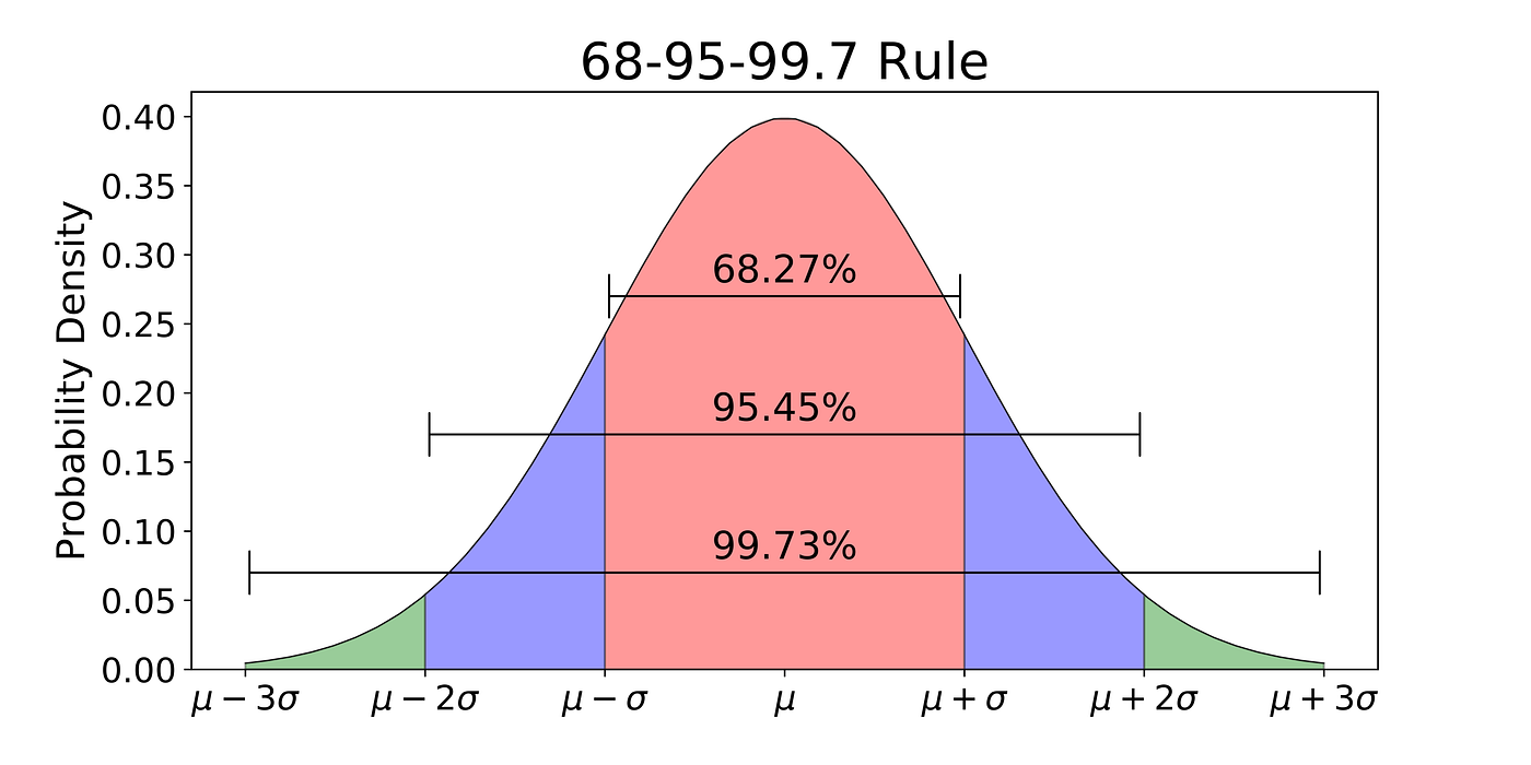
As well know, plus or minus (1,2) sd is (66%,95%) of the area
under the normal curve. Another number of interest is that plus or
minus 1.28 sd is 90% of the mass. This means that one standard
deviation is 90% of the mass divided by (1.28*2)=2.56. Hence,
to compute something analogous to sd from any distribution,
sort it and look at the 90th and 10th percentile.
def var(i): return (i.per(.9) - i.per(.1)) / 2.56
What you have to write is unsuper and merge
- Notes on
Unsuper- It cannot break ranges uness the i-th+1 value is different to the i-th value
- It cannot break unless the break contains more than
iotaitems - It cannot break unless the max and min value in that break differ by more than
sqrt(N)of all the items. - It cannot break unless there are enough items (
sqrt(N)) after the break (so we can break some more, latter)
- Notes on
merge- Merge looks at item[n] and item[n+1] in the ranges found by unsuper
- If these two adhacent items are "dull" then we merge then, and jump on to look at n+2 and n+3.
- If they are not dull, then item[n] gets added to a tmp output list and we jump on to look at n+1 and n+2
- If any merges are made, then we call merge(tmp) to see if the merged ranges can be further merged.
- Else, we return the original ranges.
As to what "dull" means, if the variability of a merge is about the same as before the merge, then we combine the two items:
  a = b4[j]
  if j < len(b4) - 1:
    b = b4[j+1]
    cy = a.y.merge(b.y)
    if cy.var()*.95 <= (a.y.var()*a.n + b.y.var()*b.n)/(a.n + b.n):
       # then merge a,b
Note that I use a Sym instance to count the symbols and computer the variance
and do the merging (which explans the arcane code shown above).
class Sym:
  def merge(i,j):
    "Copy: merge two symbol counters"
    k = Sym(n=i.at, s=i.txt)
    for x,n in i.has.items(): k.add(x,n)
    for x,n in j.has.items(): k.add(x,n)
    return k

  def var(i):
    "Query: variability"
    return - sum(v/i.n * math.log2(v/i.n) for v in i.has.values())