
home ::
syllabus ::
timetable ::
groups ::
moodle(591,
791) ::
video tbd ::
© 2021
Ethically Speaking, the Best Thing You Can Do with Most Data is Throw Most of it Away
Repeat until no crap: cut the crap
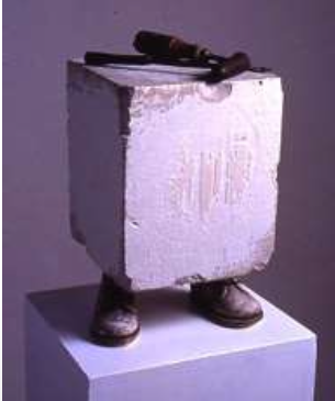
"Every block of stone has a statue signal inside it and it is the taks of the scultpro to discover it. "
-- Michelangelo some bald guy
“Perfection is achieved when there is nothing left to take away.”
-- Antoine de Saint-Exupéry
"Less, but better."
-- Dieter Rams
"In most applications examples are not spread uniformly throughout the instance space, but are concentrated on or near
a lower-dimensional manifold. Learners can implicitly take
advantage of this lower effective dimension."
-- Pedro Domingoes
Ethical systems should be debatable.
- data engagement meetings : 4 people in a room arguing and improving what they are seeing.
While it is now possible to automatically analyze such data with data miners, at some stage a group of business users will have to convene to interpret the results (e.g., to decide if it is wise to deploy the results as a defect reduction method within an organization).
- These business users are now demanding that data mining tools be augmented with tools to support business-level interpretation of that data.
- For example, at a recent panel on software analytics at ICSE’12, industrial practitioners lamented the state of the art in data mining and software engineering. - Panelists commented that “prediction is all well and good, but what about decision making?”.
- That is, these panelists are more interested in the interpretations that follow the mining, rather than just the mining.
The problem with interpretataion is that it is time- consuming and expensive.
- According to Brendon Murphy, Microsoft (UK), the high cost of interpretation implies that there is never enough time to review all that defect data or all the models generated by the data miners.
- Murphy spends much time discussing data mining and software project defect data with business users.
- He is very interested in methods that reduce the number of features and examples that need to be discussed with users.
- These reduction methods are a black art.
In the summer of 2011 and 2012, Menzies spent two months working on-site at Microsoft Redmond, observing data mining analysts.
- He observed numerous meetings where Microsoft’s data scientists and business users discussed logs of defect data.
- There was a surprising little inspection of the output of data miners as compared to another process, which we will call peeking.
- In peeking, analysts and users spend much time inspecting and discussing small samples of either raw or exemplary or synthesized project data.
- For example, in data engagement meetings, users debated the implications of data displayed on a screen.
- In this way, users engaged with the data and with each other by monitoring each other’s queries and checking each other’s conclusions.
Cluster + contrast was another peeking method seen at Microsoft.
- In this method, data was reduced to a few clusters and users were then just shown the delta between those clusters (a technique we first saw used by Sauvik Das).
- While contrasting, if feature values are the same in both clusters, then these were pruned from the reports to the user.
- In this way, very large data sets can be shown on one PowerPoint slide.
- Note that cluster+contrast is a tool that can be usefully employed within data engagement meetings.
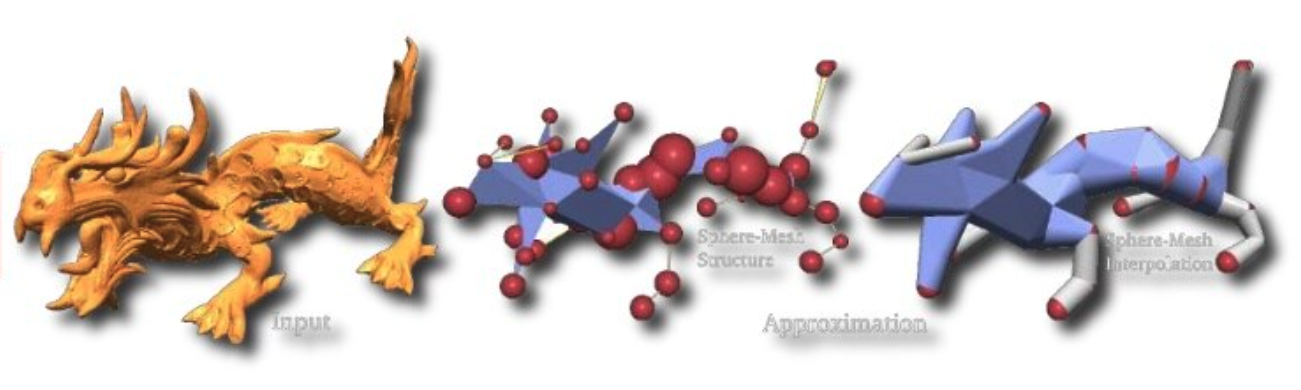
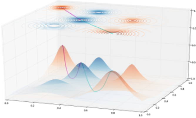
More generally, this process is mabsed on the manifold assumption (used extensively in semi-supervised learniing) that higher-dimensional data can be maped to a lower dimensional space without loss of signal.
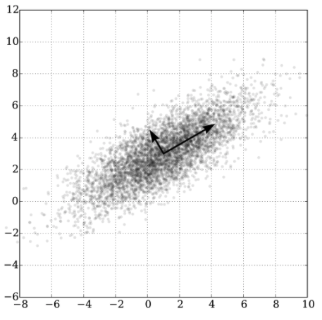
- In the following examples, the first atttributes already occuring in the domain and the second uses an attribute synthesized from the data (the direction of greates spread of the data)
Apart from simpler expalantions (and hence more user engagment and more auditability), throwing data away has privacy implications.
- Instead of sharing all data, if only share the reduced data set, then all the non-shared information is 100% private, by definition.
- Also, if we deploy systems based on the reduced set, then we never need to collect the attributes removed by pruning.
- So less intrusion into people's lives
- Fayola Peters used cluster + contrast to prune, as she passed data around a community.
- At east step, and anomaly detector was called about members of that community only added in theor local data that was not already in the shared cache (i.e. only if it was anomalous).
- She ended up sharing 20% of the rows and around a third of the columns. 1 - 1/5*1/3 thus offered 93% privacy
- As for the remaining 7% of the data, we ran a mutator that pushed up items up the boundary point between classes (and no further). Bu certain common measures of privacy, that made the 7% space 80% private.
- Next ecct 93% + .8*7 = 98.4% private,
In summary
- The Best Thing You Can Do with Most Data is Throw it Away.
- A lot of ethical functionality comes from distance and dimension functions. So lets code those.
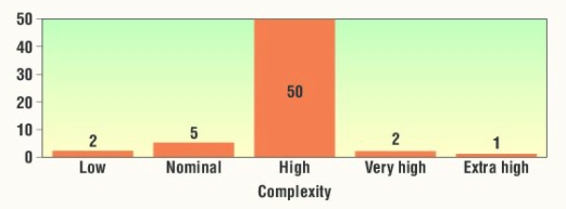
Question: is highly complex software slower to build?
Answer: the question is irrelevant (at some sites)
So what else can we throw away.
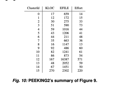
Papakroni argued that, for that purpose, you do not need to show models... just insightful samples from the domain.
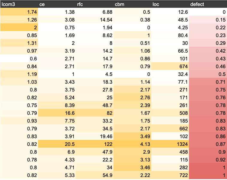
For example, here's PEEKING2’s summary of POI-3.0. The original data set is reduced from 442 rows and 21 columns to 21 rows and 6 columns.
| name | what | notes |
|---|---|---|
| lcom3 | cohesion | if m,a are the number of methods,attributes in a class number and µ(a) is the number of methods accessing an attribute,then lcom3 = (mean(µ(a)) - m)/ (1 - m) |
| ce | efferent couplings | how many other classes is used by the specific class |
| rfc | response for a class | number of methods invoked in response to a message to the object. |
| cbm | coupling between objects | total number of new/redefined methods to which all the inherited methods are coupled |
| loc | lines of code | |
| defect | defect | Binary class. Indicates whether any defect is found in a post-release bug-tracking system. |
And we know how to change these
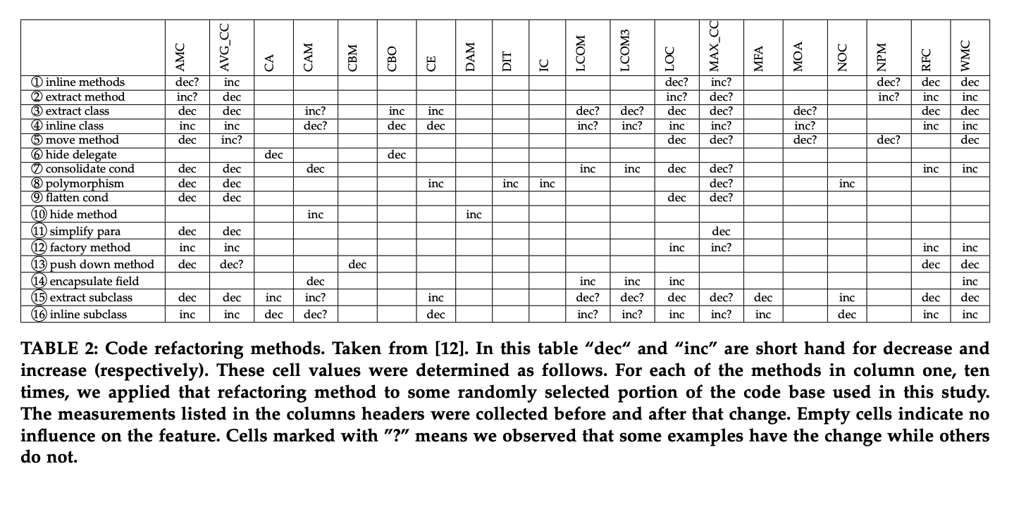
Btw, see the colors?
- One surprisingly good defect predictor is "count how often an example has attribute values falling into the worst part of each column" (e..g which side of the emdian your fall).
- And this does not even need clss labels to impement.
- Defeats most other unsupervised methods (at least, on SE data). See IVSBC in Fig8.
- And rrecently we've found it useful to look at just a few (2.5% ) of the data labels to refine what we mean by "worst half"
Here is Aha's instance-based distance algorithm, section 2.4.
(Note: slow. Ungood for large dimensonal spaces. We'll finx that below.)
L-norm (L2):
- D= (∑ (Δ(x,y))p))1/p
- euclidean : p=2
But what is Δ ?
- Δ Symbols:
- return 0 if x == y else 1
- Δ Numbers:
- x - y
- to make numbers fair with symbols, normalize x,y 0,1 using (x-min)/(max-min)
What about missing values:
- assume worst case
- if both unknown, assume δ = 1
- if one symbol missing, assume δ = 1
- if one number missing:
- let x,y be unknown, known
- y = normalize(y)
- x = 0 if y > 0.5 else 1
- Δ = (x-y)
In the following recall the Sample keeps column headers sperately
for the self.x (independent) columns and the
self.y (dependent) columns.
function Sample:dist(row1,row2,the,       a,b,d,n)
  d,n = 0,1E-32
  for _,col in pairs(self[the.cols]) do -- default. the.cols="x"
    n   = n + 1
    a,b = row1[col.at], row2[col.at]
    if    a=="?" and b=="?"
    then  d = d + 1
    else  d = d + col:dist(a,b)^the.p end end
  return (d/n)^(1/the.p) end
Distance for Symbols:
function Sym:dist(x,y)
  return x==y and 0 or 1 end
Distance for Numbers:
function Num:dist(x,y)
  if     x=="?" then y=self:norm(y); x = y>.5 and 0 or 1
  elseif y=="?" then x=self:norm(x); y = x>.5 and 0 or 1
  else               x,y = self:norm(x), self:norm(y) end
  return math.abs(x-y) end

function Num:norm(x,    a)
  if x =="?" then return x end
  return (x-self.lo) / (self.hi - self.lo + 1E-32) end
Btw, distance calcualtions are really slow
- heuristic for faster distance: divde up the space into small pieces (e.g. &sqrt;(N)
- Space between pieces = &infty;
- Space inside pieces: L2
E.g. mini-batch k-means
- Pick frist 20 examples (at random) as controids
- for everything else, run thrugh in batches of size (say 500,2000,etc)
- mark each item with its nearest centroid
- betweetn batch B and B+1, move centroid towards its marked examples
- "n" stores how often this centroid has been picked by new data
- Each item "pulls" its centroid attribute "c" towards its own attribute "x" by an amount weighted
c = (1-1/n)*c + x/n. - Note that when "n" is large, "c" barely moves at all.
Distance gets weird for high dimensions
- for an large dimensional orange, most of the mass is in the skin
- volume of the space increases so fast that the available data become sparse.
- amount of data needed to support the result grows exponentially with dimensions
- "Generalizing correctly becomes exponentially harder as the dimensionality (number of features) of the examples grows, because a fixed-size training set covers a dwindling fraction of the input space. Even with a moderate dimension of 100 and a huge training set of a trillion examples, the latter covers only a fraction of about 10−18 of the input space"
- "Our intuitions, which come from a three-dimensional world, often do not apply in high-dimensional ones. In high dimensions, most of the mass may not be near the mean, but in an increasingly distant “shell” around it; and most of the volume of a high-dimensional orange is in the skin, not the pulp."
Example of crazy high dimensiona effects:
- A large N-dimensional unit sphere (radius=1) has infitely small volume.
- V(2)= circle = πr2
- V(3)= sphere = 4/3πr3
- V(n) = hypersphere = 2πr2 * V(n-2) / n
- at r=1,n=6, V(n) > V(n-2)
- but after r=1,n=7 V(n) < V(n-2)
- Why? well for unit spheres (where r=1) L2 says ((a1-a2)2 +(b1-b2)2 + (c1-c2)2 + .... )1/2
- Q: How to maintain r=1 as the number of dimensions icnreasea?
- A: Minimize all the gaps (a1-a2), (b1-b2), (c1-c2), etc
- So for constant radius, as dimensions grows, the gap betweeen examples has to shrinl
- Practical consueqeucenes: as models get more complex, the space of relevant (i.e. nearby) examples gets vanishingly small
- Good news: only need to search in nearby region for relevant data
- Bad news: models are either low-dimensional or can't be modeled (not enough relevant data)
- Better news: the models that can be modeled conform to the manifold assumption.
Q: How to find those lower dimensions?
A: Let them find you.
-
mutliple times, take randoms steps across the space
-
technique used to reduce the dimensionality of a set of points
-
known for their power, simplicity, and low error rates when compared to other methods
-
if n randomly selected dimension say you are similar to something else
- then you are probably similar
-
"Fortunately in most applications examples are not spread uniformly throughout the instance space, but are concentrated on or near a lower-dimensional manifold. "
-
"For example, k-nearest neighbor works quite well for handwritten digit recognition even though images of digits have one dimension per pixel, because the space of digit images is much smaller than the space of all possible images."
-
"Learners can implicitly take advantage of this lower effective dimension"

- Method one: Guassian random projections
- Matrix = rows * cols
- Matrix A,B
- A = m × n
- B = n × p
- C = A*B = m x p
- So we can reduce n=1000 cols in matrix A to p=30 cols in C via a matrix
- 1000 row by 30 cols
- Initialize B by filling each column with a random number pulled from a normal bell curve
- Only works for numbers
- Requires all the data in RAM (bad for big data sets)
- Method two: LSH: locality sensitivity hashing
- Find a way to get an approximate position for a row, in a reduced space
- e.g. repeat d times
- Find two distant (*) "pivots" = (p,o)
- Pick, say, 30 rows at random then find within them, the most distant rows
- the i-th dimension:
- this row's d.i = 0 if (row closer to p than o) else 1
- Find two distant (*) "pivots" = (p,o)
- repeat d=log(sqrt(N))+1 pivots to get d random projectsion
- e.g. repeat d times
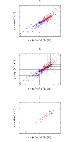
- If you want not 0,1 on each dimension but a continuous number then:
- given pivots (p,o) seperated by "c"
- a = dist(row,p)
- b = dist(row,o)
- this row's d.i = (a^2 + c^2 - b^2) / (2c)
- Cosine rule
- Can be done via random sampling over some of the data.
- Better for bigger data
- But less exact
- still, darn useful
- Find a way to get an approximate position for a row, in a reduced space
(*) beware outliers :
- A safe thing might be to sort the pivots by their distance and take something that is 90% of max distance
For the data sets process last time
- Implement the Aha distance function for
Nums andSyms - For each row item
- print it
- print its nearest item (that is not it) and the distance to it (this will be a number 0..1)
- print its furtehst item and the distance to it (this will be a number 0..1)
function Sample:neighbors(r1,the, rows,       a)
  a = {}
  rows = rows or self.rows
  for _,r2 in pairs(rows or self.rows) do
    a[#a+1] = {self:dist(r1,r2,the) -- item1: distance
              ,r2} end              -- item2: a row
  table.sort(a, function (y,z) return y[1]<z[1] end)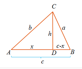
return a endShow the derivation of the cosine rule. Given two items A,B sepeated by distance c,
- given a third item C of disance a,b to B,A
- derive an expression for x being the distance that that C falls along the line between East and West
- Hint1: Pythagoras
- Hint2:
Using the cosine rule, implement random projects.
Firstl, omplement faraway, a function that selects the.samples=128 rows (at random) then finds the thing the.far=.9 of the distance to furthest.
function Tbl:faraway(row,the,cols,rows,      all)
  all = self:neighbors(row,the,
                       shuffle(self.rows, the.samples)) -- some, picked at random
  return all[the.far*#all // 1][2] end
Implement div1 that does one random projection, based on two distant points:
function Sample:div1(the,cols,rows,         one,two,c,a,b,mid)
  one  = self:faraway(Lib.any(rows), the, cols, rows)
  two  = self:faraway(one,           the, cols, rows)
  c    = one:dist(two, the, cols)
  for _,row in pairs(rows) do
    a  = row:dist(one, the, cols)
    b  = row:dist(two, the, cols)
    row.projection = (a^2 + c^2 - b^2) / (2*c) -- from task2
  end
  rows = sorted(rows,"projection") -- sort on the "projection" field
  mid  = #rows//2
  return slice(rows,1,mid), slice(rows,mid+1) end -- For Python people: rows[1:mid], rows[mid+1:]
Implement divs that does many random projections dividing the data down to (say) sqrt(n) of the data.
Note: in the following code leafs is an accumulator passed
down the tree. When we return it, it is a list of lists
where each sublist are all the items in one leaf.
function Sample:divs(the,    leafs)
  leafs={}
  self:_divs(self.rows,0, the,leafs,cols or self.x,(#self.rows)^the.enough)
  -- table.sort(leafs) -- dont do, yet
  return leafs end

function Sample:_divs(rows,lvl,the,leafs enough,
              pre,left,right)
  if   the.loud -- very useful debugging aid
  then pre="|.. ";print(pre:rep(lvl)..tostring(#rows))
  end
  if   #rows < 2*enough
  then leafs[#leafs+1] =  rows
  else left,right= self:div1(the,cols,rows)
       self:_divs(left, lvl+1, the, leafs, enough)
       self:_divs(right,lvl+1, the, leafs, enough) end  end
Note from here, we can feature pruning in each leaf and anomaly detection to implement the ethical operators described above. Next week!
Hand in your code, in the repo, and your run times.