high level understanding of how to apply this model to new images

[kaczmarj]

hi shahira, i am writing this issue to serve as notes for myself and other readers. i am documenting how to apply this model to images.

first, i converted the consep model to torchscript for use outside of python (and to serialize the model with weights).

Code to load model trained on consep and save to torchscript

import torch
from model_arch import UnetVggMultihead

model_config = {
    "dropout_prob": 0.2,
    "initial_pad": 126,
    "interpolate": "False",
    "conv_init": "he",
    "n_classes": 3,  # lymphocytes, tumor, stroma
    "n_channels": 3,
    "n_heads": 4,
    "head_classes": [1, 3, 5*3, 21],
}

model = UnetVggMultihead(kwargs=model_config)
weights = torch.load("pretrained_models/mcspat_consep.pth", map_location="cpu")
model.load_state_dict(weights)
script = torch.jit.trace(model, torch.ones(1,3,448,448))
# Freeze the model, and do some other optimizations...
script_opt = torch.jit.optimize_for_inference(script)
# Save.
torch.jit.save(script_opt, "mcspatnet-consep-torchscript-opt.pth")

mcspatnet-consep-torchscript-opt.pth.gz

If you download the model, please gunzip it -- I gzipped the file so I could upload it here.

Here are the steps to apply the model to new data...

1. Load the model

2. Load an RGB image of tissue (500x500 pixels at 0.5 microns per pixel). @ShahiraAbousamra - is this correct?

3. Normalize the image to [0, 1] -- usually this means divide the image by 255.

4. Run the image through the model. This gives four output arrays: density map for all nuclei, density map for nuclei with associated classes, (and the next two I'm not quite sure about).

5. Apply sigmoid to the density map for all nuclei (the first output of the model).

6. Threshold the sigmoided density map (skimage.filters.filters.apply_hysteresis_threshold(density_map, low=0.5, high=0.5))

7. Find connected components in this thresholded density map (skimage.measure.label(arr))

8. Remove any connected components with an area below a threshold (threshold in the code is 5 pixels).

9. Get the center of each connected component. This point indicates the presence of a nucleus. There is no associated classification yet. That will happen in the next few steps...

       centers = np.zeros((500, 500))  # image height and width
       contours, hierarchy = cv2.findContours(density, cv2.RETR_EXTERNAL, cv2.CHAIN_APPROX_NONE)
       for idx in range(len(contours)):
           contour_i = contours[idx]
           M = cv2.moments(contour_i)
           if(M['m00'] == 0):
               continue;
           # The centroid of this prediction.
           cx = round(M['m10'] / M['m00'])
           cy = round(M['m01'] / M['m00'])

10. Softmax the second output of the model (density map for nuclei with associated classes). Softmax in the channel dimension.

11. Take the argmax along the channel dimension to get hard classes at each pixel in the image.

12. For each class...
    a. create a binary mask indicating the presence of that class: arr == class_idx
    b. multiply this binary mask against the centers array from step 9. this will zero out regions that do not have a nucleus.
    c. get the center of each point.

    dots = (arr == class_idx) * centers
    with_dots = np.where(dots > 0)
    for idx, _ in enumerate(with_dots[0]):
        cy = with_dots[0][idx]
        cx = with_dots[1][idx]

Step 9 gives the location of each nucleus. Step 12c gives the location and class of the nuclei.

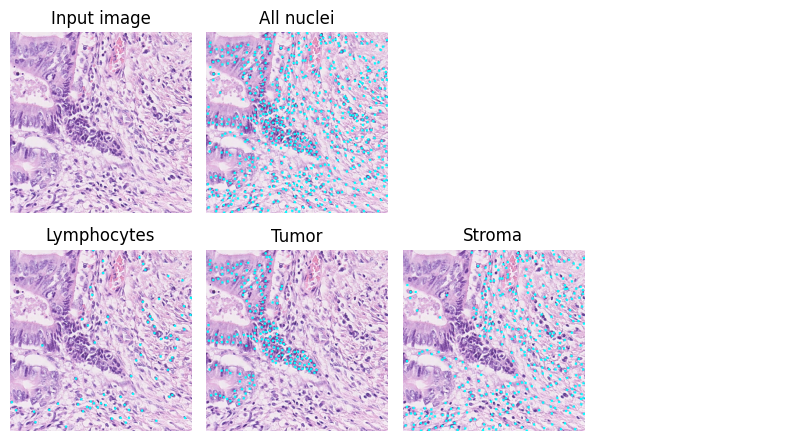
Here is an example of the results. The cyan dots show the predicted points.