[TOC]
对于分类任务,我们可以认为我们是对如下进行建模:
$$
\hat{y} = \text{arg}\max_y p(y \mid x)
$$
我们拥有 Bayes Theorem:
$$
\underbrace{P(y\mid x)}_\text{posterior}
= \frac{
\overbrace{P(x\mid y)}^\text{likelihood}
\overbrace{P(y)}^\text{prior}
}{P(x)}
$$
因此可以把问题重写为
$$
\hat{y} = \text{arg}\max_y P(y \mid x)
\longrightarrow
\hat{y} = \text{arg}\max_y P(x \mid y)P(y)
$$
如若假设
\ \therefore \hat{y} = \text{arg}\max_y P(y) \prod_i^N P(x_i \mid y) $$
对于一个文本的 BoW 表示为:

数据集被定义为文档的标签对:


graph LR
	raw[原始数据对<br>corpus : label]
	prep[预处理后的数据对<br>小写 分词 等]
	bow[BoW 表示]
	fs[特征表示<br>特定单词的统计 : label]
	raw -->|preprocessing| prep
	prep --> bow
	bow --feature<br>extraction--> fs
	prep -->|label| fs
在完成特征表示后,我们可以得到 prior(先验概率)(这可以通过聚合运算得到)。

假设训练集如上,则 prior 为
$$
\begin{cases}
P(+) = \frac{3}{5}\
P(-) = \frac{2}{5}
\end{cases}
$$
我们也可以获得 likelihood,以 good 为例
$$
P(\text{good} \mid +) = \frac{2}{4}
$$

这里涉及到的运算矩阵为上,good 出现了2次,而总词数为 4(2 good,1 movie,1 bad) $$ \begin{align*} P(w \mid c) &= \frac{\text{word }w \text{ count in class } c}{\text{total word in class } c} \ &= \frac{\text{count}(w, c)}{\sum_{x\in V} \text{count}(x, c)}
\end{align*}
$$
为防止出现计数为 0 情况,使用 Add-One Smoothing:
$$
\begin{align*}
P(w \mid c)
&= \frac{\text{count}(w, c) +1}{\sum_{x\in V} (\text{count}(x, c)+1)}
\
&= \frac{\text{count}(w, c) +1}{|V| + \sum_{x\in V} \text{count}(x, c)}
\end{align*}
$$
因此:
$$
P(\text{good} \mid +) = \frac{2}{4} \rightarrow\frac{2+1}{4+1} = \frac{3}{5}
$$

Not as good as the old movie, rather bad movie. -> Not as good as the old movie, rather bad movie.
移除了每个实例中的所有重复项。因此,单词“movie”的额外出现不会改变任何内容。
请注意,这意味着需要根据数据重新计算条件概率。
I didn’t like the movie, but it was better than Top Gun -> I didn’t NOT_like NOT_the NOT_movie, but it was better than Top Gun
对于所有 logical negation (e.g., n’t, not, no, never) 后 append NOT_ 直到下一个 punctuation。

Discriminative algorithms 学习 
损失函数通过 BCE 定义。我们先定义 neg likelihood (min neg likelihood) $$ H(P, Q) = -\sum_cP(c)\log Q(c) $$ 如有 $$ \begin{cases} P =[1, 0]\ Q_1 = [0.92, 0.08] \end{cases} $$
对于多class,用 softmax

对于不同的句子,为获得固定维度的句子文档表示

可以用平均值:

这真是个馊主意: 根据句子长度大小固定模型结构 针对特定单词位置学习模型权重
自动学习的特征 Auto Learnt Features
- 灵活适应数据中高度复杂的关系
- 但是:它们需要更多数据来学习更复杂的 patterns

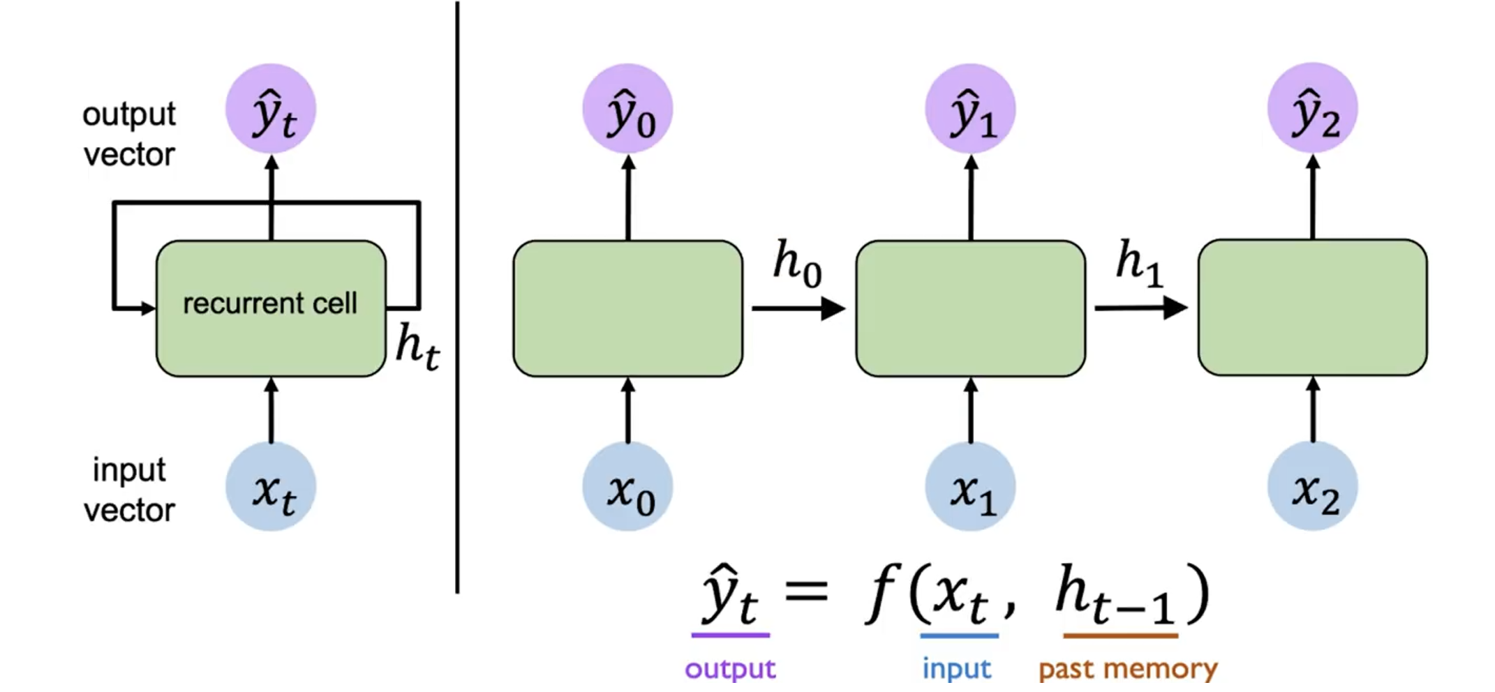
模型难以从较早的输入中学习:
-
Tanh 的导数在 0 到 1 之间
-
Sigmoid 的导数在 0 到 0.25 之间
较早层的梯度涉及同一矩阵
- 根据主导特征值(dominant eigenvalue),这可能导致梯度“消失”或“爆炸”
而由于 RNN 的循环结构,在反向传播过程中,对于
$h_0$ 计算梯度时,导致很多梯度会相乘,从而导致梯度可能会指数级地减小(消失)或增大(爆炸)。这会导致学习困难,尤其是对于长序列。如果梯度很多都
$>1$ ,则会导致梯度爆炸(考虑$1.01^{100}$ ),我们可以通过梯度裁剪(Gradient Clipping)来解决这个问题。即当梯度的范数超过一个阈值时,将梯度缩放到一个较小的范围。如果梯度很多都
$<1$ ,则会导致梯度消失,这个问题比较难解决,我们通常会使用

Filter:在一个方向上对整行(单词)进行滑动窗口
- Filter width = embedding dimension
- Filter height = normally 2 to 5 (bigrams to 5-grams)


我们不知道最后会有多少维(因为输入长度不确定),但是我们可以做的
RNNs vs CNNs(循环神经网络与卷积神经网络的对比)
- CNNs(卷积神经网络)在涉及关键短语识别的任务中表现出色(key phrase recognition)
- RNNs(循环神经网络)在需要理解长距离依赖关系时表现更好

$$ \begin{align*} F_1 &=\frac{2\cdot\text{Precision}\cdot\text{Recall}} {\text{Precision}+\text{Recall}} \ &= \frac{TP}{TP + \frac{1}{2}(FP+FN)}
\end{align*} $$


例子
- 设 A = "学生数学得 A"
- 设 B = "学生英语得 A"
- 设 C = "学生熬夜学习"
最初,数学得 A(A)和英语得 A(B)可能是独立事件 - 一个科目的成功并不一定意味着另一个科目也会成功。
但是,当我们在给定 C(熬夜学习)的条件下:
- 如果我们知道一个学生熬夜学习(C),那么数学考得不好(非 A)可能表明他们把时间花在学习英语上,这使得他们在英语上表现更好(B)的可能性更大
- 同样,数学考得好(A)可能表明他们把熬夜时间用在了数学上,这使得他们在英语上表现较差(非 B)的可能性更大
我们可以用数学表达式来表示这一点: 虽然
$P(A,B) = P(A)P(B)$ (独立性) 但我们可能发现$P(A,B|C) \neq P(A|C)P(B|C)$ (条件依赖)被称为伯克森悖论或碰撞偏差。