-
matplotlibis the most commonly used library for making scientific figures- NOTE: Some of the official
matplotlibdocumentation is out of date - For help, it's best to look for up-to-date tutorials
- NOTE: Some of the official
-
If you haven't already, install
matplotlib -
We'll also use
numpytoday, so you should have that installed already.- It would also be a good idea to become familiar with numpy arrays
-
For almost all the plotting you'll do, you only need this
importline at the topimport matplotlib.pyplot as plt -
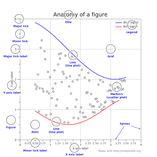
matplotlibuses a hierarchy of elements in the figure that can be manipulated independently.
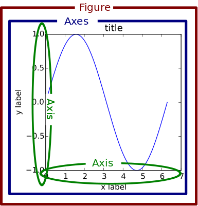
-
Figuredenotes the entire plotting areas -
An
Axesis a subplot within a figure. -
Each
Axesthen has a bunch of elements that can be adjusted individually.
-
There are different ways to interact with and adjust plots, but we'll use what's called the "object-oriented approach". Basically this just means that we keep track of and interact with each element of a plot individually. To adjust an element, we call some method associated with that element.
-
Let's walk through this example taken from the Real Python site.
import numpy as np import matplotlib.pyplot as plt # Look up the numpy documentation. What are these functions doing? rng = np.arange(50) rnd = np.random.randint(0, 10, size=(3, rng.size)) yrs = 1950 + rng # What's going on here? What is the .subplots() function returning? # What is the figsize argument setting? fig, ax = plt.subplots(figsize=(5, 3)) # This is a fake dataset, but how is it using the values generated with numpy? ax.stackplot(yrs, rng + rnd, labels=['Eastasia', 'Eurasia', 'Oceania']) # What sorts of plot elements are we setting? ax.set_title('Combined debt growth over time') ax.legend(loc='upper left') ax.set_ylabel('Total debt') ax.set_xlim(xmin=yrs[0], xmax=yrs[-1]) # What is this doing? fig.tight_layout() # Actually displays figure plt.show() -
What if you want to create a figure with more than one subplot?
fig, ax = plt.subplots(2,2) # What does ax look like after this function call? ax[0,0].stackplot(yrs, rng + rnd, labels=['Eastasia', 'Eurasia', 'Oceania']) ax[0,1].stackplot(yrs, rng + rnd, labels=['Eastasia', 'Eurasia', 'Oceania']) ax[1,0].stackplot(yrs, rng + rnd, labels=['Eastasia', 'Eurasia', 'Oceania']) ax[1,1].stackplot(yrs, rng + rnd, labels=['Eastasia', 'Eurasia', 'Oceania']) plt.show() -
What are some of the built-in plot types in
pyplot?-
Example plots: https://matplotlib.org/tutorials/introductory/sample_plots.html
Pick two plot types from this gallery, figure out how to plot them, and
create a figure with both plots on it.
-
    - Use `matplotlib` to create some plot that we did not cover in class.
      - Try to find a plot that will be relevant to your final project.

    - Create a pseudocode outline for the overall structure of your final project.

    - Start filling out as much code as possible under your pseudocode outline. Flag areas where you are stuck or aren't quite sure how to proceed.
-
Numpy arrays are specialized data structures for storing and manipulating multi-dimensional sets of values. Note that we've done some simples versions of this with lists of lists, but these lack any associated methods.
-
Here's how we stored a 2-dimensional array using just standard Python lists
myBasicArray = [[3,5,8],[9,12,14]] -
Here's the syntax to access the number in "row 2, column 2"
myBasicArray[1][1] -
Here's our list-of-lists array printed to screen
print(myBasicArray) -
However, if we want to do anything other than access or change these values, we would need to write custom functions to do so.
-
Here's how we could store these same values as a numpy array. Remember that we still need to precede numpy functions with
np. Note that thearray()function requires a single list as an argument.import numpy as np myArray = np.array([[3,5,8],[9,12,14]]) -
We start to notice differences from lists of lists as soon as we print our array.
print(myArray) -
Conveniently, numpy prints out the array in a matrix-like way.
-
There are some built-in functions to create numpy arrays with either all 0s or all 1s, or a range of values.
myAllZeroArray = np.zeros( (3,5) ) print(myAllZeroArray) myAllOneArray = np.ones( (5,3) ) print(myAllOneArray) myRangeArray = np.linspace(2,11.5,20) print(myRangeArray) # linspace gives a specified number of values in the given interval -
Now, let's say that we want to turn our one-dimensional array into an multi-dimensional array. Conveniently, numpy arrays have a built-in function to do this - called reshape().
myRangeArray = myRangeArray.reshape( 2,10 ) print( myRangeArray ) myRangeArray = myRangeArray.reshape( 4,5 ) print( myRangeArray ) -
Multi-dimensional arrays can also easily be transformed. For instance, let's say we want to flip an array along its left-to-right axis.
myRangeArray = np.fliplr(myRangeArray) print( myRangeArray ) -
The power of numpy arrays becomes immediately apparent if we want to transform all the values in our array in some way. For instance, let's say we want to subtract a constant value from every element. All we have to do is write the operation with the array.
print( myRangeArray-1 ) print( myRangeArray*2 ) print( myRangeArray**2 ) -
These operations would not be possible as written with our basic list-of-lists array.
myBasicArray-1 # Fail -
You can also evaluate boolean statements on all elements in an array.
print( myRangeArray % 2 == 0 ) # Find even numbers -
Built-in functions are also available that operate on all elements of an array.
print( myRangeArray.sum() ) print( myRangeArray.min() ) -
Array axes can be indexed independently to extract particular sets of values. For instance, let's say we want all values in the 3rd column.
print( myRangeArray[ : , 2] ) -
Multiple numpy arrays can be combined in different ways. For instance, if we wanted to stack arrays on top of one another, we can use the vstack() function.
print( np.vstack( (myAllZeroArray,myAllOneArray.reshape(3,5)) ) )
-
A population consists of all members of a given set (e.g., all LSU students). We often want to understand something about a population (e.g., amount of student debt), but it can be very difficult (impossible) and time consuming to get this information from everyone. Instead, we take a sample from this population, calculate the statistic of interest for the sample, and use it to try and understand the population as a whole.
-
Ideally, the sample is randomly drawn from the entire population. The more members of the population are included in the sample, the more confident we can be that our sample statistic accurately reflects the entire population. But just how much uncertainty is there in our estimate for a given sample size? This is a fundamental question in the field of statistics.
-
If we know that the quantity of interest in the population has a certain distribution (e.g., Normal), we can sometimes just apply a known formula to tell us how confident we should be. But when the underlying distribution in the population is unknown, we rely on a procedure called bootstrapping.
-
One of the simplest and most useful things we can do with (pseudo-)random numbers is draw values from a dataset.
-
We can draw these values in two ways - with or without replacement. If we sample without replacement, we are just reordering the dataset. Each time we sample a value, we cannot sample it again.
data = np.array([ 0.82803637, 0.00382416, 0.07481507, 0.99684717, 0.99995017, 0.63965781, 0.99360978, 0.3625829 , 0.99999972, 0.98201947, 0.00118308, 0.52392163, 0.95489943, 0.45001676, 0.65437422, 0.94684642, 0.0114679 , 0.94362976, 0.0704053 , 0.27266416]) data = np.random.choice(data, size=20, replace=False) print(data) data = np.random.choice(data, size=20, replace=False) print(data) # In these cases, each value in the original dataset is only present # once in the resampled datasets. -
When we sample with replacement, some values may be sampled multiple times and others sampled not at all. Replacement means that when we sample a value, we put it back into the pool with the potential to be sampled again.
print( np.random.choice(np.array([1,2,3,4,5]), size=5, replace=True) ) print( np.random.choice(np.array([1,2,3,4,5]), size=5, replace=True) ) print( np.random.choice(np.array([1,2,3,4,5]), size=5, replace=True) ) print( np.random.choice(np.array([1,2,3,4,5]), size=5, replace=True) ) print( np.random.choice(np.array([1,2,3,4,5]), size=5, replace=True) ) -
One application of sampling with replacement is a procedure called "bootstrapping". The name comes from the phrase "pull yourself up by your bootstraps" and applies when we are trying to learn something about data drawn from an unknown distribution. To start, let's take a look at our data...
import matplotlib.pyplot as plt plt.hist(data) plt.show() -
Now, let's say we're interested in learning about the mean of the population from which we've sampled these values
dataMean = np.mean(data) print( dataMean ) -
The data don't obviously come from a standard distribution, so it's difficult to know how confident we should be in our estimate of the mean. Bootstrapping is one way around this. We can draw a series of samples with replacement from our data and calculate their means. This collection of means gives us an idea of how confident we can be in our estimate.
# Number of bootstrap replicates - more is better, but takes longer bootNumber = 1000 # array to store results of bootstrapping meanBoots = np.array([]) # For loop to perform bootstrapping for _ in range(bootNumber): # Draw new bootstrap replicate samp = np.random.choice(data, size=data.size, replace=True) # Calculate mean from each replicate meanBoots = np.append(meanBoots,np.mean(samp)) # Examine bootstrap distribution on the mean plt.hist(meanBoots) plt.show() -
If the number of bootstrap replicates is reasonably large, the distribution of bootstrap means should look roughly Normal (bell-shaped), even though our "data" are very non-Normal. This phenomenon is explained by the Central Limit Theorem.
-
While visually inspecting the distribution of bootstrap means is useful, we'd also like to get a quantitative estimate of our uncertainty. To do this, we can generate an estimate of a confidence interval, typically a 95% confidence interval. This interval tells us that if we were to re-sample from our population many times, the means from these samples would fall in this interval 95% of the time.
# First, we need to sort the means from our bootstrap replicates so that # the smallest values are at the beginning and the largest values are at # the end. meanBoots = np.sort(meanBoots) # Find the values in our sorted list that exclude the lowest 2.5% and the highest 2.5% (for a total of 5%). # This code looks a bit intimidating, but let's take a closer look: # bootNumber*0.025 - Calculate the value corresponding to 2.5% of our bootstrap replicates. # np.floor() - Take the number from above and round down. # np.int() - Take the rounded number and convert it from a float to an int. # meanBoots[] - Use that int to find the appropriate value from the set of bootstrap means. confInterval_95 = (meanBoots[np.int(np.floor(bootNumber*0.025))],meanBoots[-1*np.int(np.floor(bootNumber*0.025))]) -
Ok, here's a similar dataset that's 10x as big as the first one. Estimate a bootstrap confidence interval for this dataset and see how it compares.
bigData = np. array([ 4.43916145e-01, 9.79508118e-01, 1.55889064e-01, 8.12968915e-01, 9.40903388e-01, 8.25403668e-01, 9.05186425e-01, 5.31823942e-01, 6.97253335e-02, 5.68562579e-01, 9.98353836e-01, 9.65390694e-01, 3.25003333e-02, 1.60461982e-02, 5.90021669e-01, 9.91478219e-01, 9.99995554e-01, 8.34818349e-01, 2.32329999e-01, 3.14276138e-01, 9.91165289e-01, 2.82183381e-01, 9.99528439e-01, 9.99348785e-01, 2.88281673e-01, 4.78383293e-02, 2.64463949e-02, 1.05601730e-01, 5.01204150e-01, 4.02865627e-01, 9.40431746e-01, 9.99984702e-01, 9.93685144e-01, 9.72354842e-01, 4.81530907e-01, 5.85902306e-01, 9.77466650e-01, 9.91940398e-01, 9.45839706e-01, 4.83826810e-01, 7.35641408e-01, 9.99999178e-01, 7.49026507e-01, 1.41951172e-01, 9.95191929e-01, 9.59170673e-01, 9.99973726e-01, 9.84827026e-01, 6.15954796e-03, 2.13938395e-01, 9.99983405e-01, 2.23600231e-01, 4.62689186e-03, 9.78762820e-01, 9.47722497e-03, 2.99886037e-03, 7.76948811e-01, 9.71141767e-01, 1.89345673e-01, 9.99011748e-01, 9.99960501e-01, 9.91306150e-01, 5.87503957e-01, 3.72923339e-01, 9.97353144e-01, 2.39760063e-02, 9.47302543e-01, 9.99407204e-01, 8.75762742e-01, 3.50833284e-01, 9.00166070e-01, 7.47229948e-01, 9.82860841e-01, 5.31726216e-01, 4.96990082e-01, 8.14009214e-02, 7.41329364e-02, 9.06052786e-01, 9.94765084e-01, 5.16281555e-01, 4.12539687e-01, 2.80712864e-01, 9.98294713e-01, 2.57042242e-01, 7.69605838e-01, 6.93744267e-01, 8.05010371e-02, 7.39394253e-01, 7.72264097e-01, 9.95796109e-01, 9.52355244e-01, 5.70491625e-02, 9.53184390e-01, 9.76624195e-01, 7.48503624e-01, 5.93468779e-01, 8.21453632e-01, 3.80685289e-01, 3.70567641e-01, 8.82285740e-01, 1.11559343e-01, 9.94547968e-01, 9.99984325e-01, 8.36954301e-01, 9.99349401e-01, 9.97728378e-01, 7.85442833e-01, 8.43647238e-01, 9.99999995e-01, 9.99438025e-01, 2.84201700e-01, 9.86931089e-01, 1.10653055e-01, 9.34485365e-01, 9.99667966e-01, 2.24889351e-01, 3.67507765e-02, 9.99976347e-01, 2.54474090e-01, 8.70004892e-01, 7.94592422e-02, 7.45083565e-01, 1.17011723e-01, 6.71071293e-01, 9.22324095e-01, 1.84300134e-02, 1.34330579e-01, 9.98649102e-01, 3.13750127e-02, 9.85101141e-01, 7.92027220e-02, 1.19253219e-01, 9.95017422e-01, 1.36305372e-01, 1.47265279e-02, 5.77995717e-01, 8.60895269e-01, 4.20207824e-01, 6.45650066e-01, 9.99964337e-01, 9.08686187e-01, 4.64678083e-02, 3.62104537e-01, 1.79003729e-02, 4.43108085e-01, 3.25369371e-01, 8.35032692e-01, 4.11413844e-01, 4.30082001e-01, 8.61812507e-01, 9.99592911e-01, 7.23206231e-01, 9.72971197e-01, 9.40323368e-01, 9.91770643e-01, 9.98079598e-01, 3.99557117e-01, 9.76504268e-01, 1.09519946e-05, 9.68713617e-01, 9.12709727e-01, 9.43075658e-01, 1.01931539e-01, 5.97167579e-04, 5.09379061e-02, 2.27517938e-01, 1.35128089e-01, 8.01243513e-01, 9.95445201e-01, 6.48027461e-01, 8.68050299e-01, 9.99990707e-01, 9.98065105e-01, 4.88803544e-02, 9.95784501e-01, 1.90950945e-01, 7.77998449e-02, 9.96819921e-01, 1.02749474e-01, 9.73309097e-01, 9.51092346e-01, 5.96272519e-01, 8.74382355e-01, 9.84488061e-01, 2.36875593e-01, 9.65365939e-01, 9.18195078e-01, 9.97692900e-01, 9.73600579e-01, 2.10149361e-01, 1.51508937e-03, 9.57615474e-01, 6.13810640e-01, 8.19255768e-01, 9.93310944e-01, 9.92655501e-01, 9.94268680e-01, 9.88436729e-01, 9.72657802e-01, 8.33891126e-01])