5-1-HypothesisTestingWithLinearModels.Rmd

# Rescaling our Data with Z-Scaling

If any sample can be described in terms of a mean and standard deviation, then it 
follows that any observation within that sample can also be described in terms of
its value relative to that sample's mean and standard deviation.  Describing your
data in this way is caled *"re-scaling"* your data, and is used to make it simpler to
compare samples with different scales, or even different units.  


To see z-scaling in action, let's look at the histograms of two different variables:
`x1` and `x2`.  Since they have a lot of data, let's not bother with binning; 
just plot their histograms using the `plot(density(x))` and `lines(density(x))` functions:
```{r}
set.seed(120)
x1 <- rnorm(5000, mean=35, sd=12)
x2 <- rnorm(5000, mean=50, sd=20)

```

Notice that the two distributions have different means and width.  Now, let's rescale them
so their data points are more directly comparable:. 

$$ Z = \frac{X - \bar{X}}{s}  $$
(Note: notice any similarity between this and the effect size calculations we did before?)

Re-scale the data below and plot their two density plots.  How do they compare now?
```{r}
# plot(density((x1 - mean(x1)) / sd(x1)))
# lines(density(scale(x2)))

pt(2, length(x1) - 1)
y <- rnorm(500)
qqnorm(y, alpha=0.5)
qqline(y)
```


This operation is so common, that R has it as a built-in function: `scale()`.  Try it out 
and verify that it gets the same values and the same density plots as the equation we did 
above (note: it will return a column of results, instead of a single vector.  Get the vector by indexing: `x[,1]`:
```{r}

```


Now, even though this is technically called `Z-Scaling` the data (since the Z-distribution is
described simply with the mean and standard deviation, just like this dataset does), it does
*not* mean that z-scaling your data will make it have a Z-distribution.  Let's verify that with a uniform distribution.
Plot the z-scaled density distribution of a uniformly-distributed dataset with 5000 points:
```{r}

```

However, if your data does happen to be z-distributed (also called the `normal distribution`), 
then we can say things about any point of our dataset just by comparing its z-scaled value to the theoretical 
normal distribution!  Let's try it out below by answering the following questions and
seeing if the results are *similar*:

What percentile of the data is located at Z=0, Z=0.5, and Z=1.5?
```{r}

```

Using the `pnorm()` function, what percentile would be *expected* to be located
at Z=0, Z=0.5, and Z=1.5?  Are these results similar to our dataset?
```{r}

```

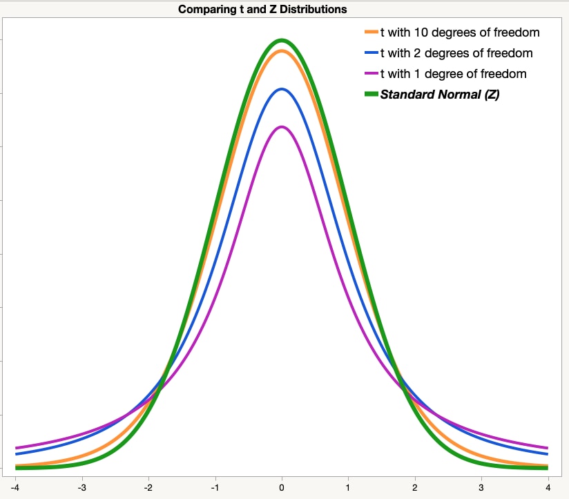
There is an issue with our dataset that prevents us from simply using the normal distribution;
it's the same issue that has plagued us through the whole class: 
*our standard deviation is estimated from our sample mean, not the true mean*.  This means
we can't divide by N, but by N-1.  As a consequence, we end up with a slightly-different
distribution that is affected by our degrees of freedom: the *"t distribution"*.

As the number of degrees of freedom approaches infinity, the t-distribution's shape approaches
the Z-distribution's shape.

![](https://www.jmp.com/en_us/statistics-knowledge-portal/t-test/t-distribution/_jcr_content/par/styledcontainer_2069_1940499363/par/image.img.png/1580489179006.png)
So, let's correct our estimate by checking the expected percentile value against the
t distribution, using the `pt()` function.  Is it closer to what we observed?
```{r}

```



We can replicate the figure above by using the `dnorm()` and `dt()` functions.
Let's try it!  Compare the Z and t distributions with different degrees of freedom.
At what degrees of freedom does the t distribution "basically" match the z distribution?
```{r}

```



# Hypothesis Testing with a T-Test

**Scenario**: 20 patients participated in a repeated-measures sleep study, where the amount of deep sleep they experienced
before receiving a treatement (M=153.8, SD=26.3) and after they received a treatment (M=186.3, SD=66.3) were compared.  
It was found that, on average, the patients had 30.5 minutes more deep sleep after the treatment than before the treatment 
(SD=38.8, d=0.79, t(9)=2.5, p<.001).  


For this study, we're going to set two goals:
  *Goal 1*: That before the treatment, the patients as a group were suffering from an abnormal amount of sleep.
     For this (fictional) protocol, the medical community considers a "normal" amount of sleep to be 180 minutes.
   *Goal 2*: We want to conclude that the treatment *didn't do nothing* to the amount of deep sleep the patients obtained.
     (Yes, this is a funny way to describe the results. Such is hypothesis testing!)


Dataset (just run the code below):
```{r}
set.seed(42)
deepsleep.before <- rnorm(20, 150, 30)
deepsleep.after <- deepsleep.before + 40 + rnorm(20, 0, 35)
```

Before we start, let's verify that the data matches the description above.  
Using the `paste()` function, print the following message using values you calculated
from the data:
Before Treatment: M = 155.8 ; SD = 39.4 
<!-- After Treatment: M = 186.3 ; SD = 66.3  -->
Inter-Treatment Difference: M = 30.5 ; SD = 38.8 ; d = 0.79 
```{r}

```

## Goal 1: Compare the distribution of before-treatment sleep times to a known value (One-Sample t-test)

*Goal 1*: That before the treatment, the patients as a group were suffering from an abnormal amount of sleep.
     For this (fictional) protocol, the medical community considers a "normal" amount of sleep to be 180 minutes.
     
     
Since our data was sampled from a normal distribution, let's rescale the data and find out what percentile 
on the `t` distribution our data lies!  The formula for this (use the standard deviation for $\widehat\sigma$)

$$ t = \frac{Z} {s} = \frac{\bar{X} - \mu}{\widehat\sigma / \sqrt{n}}$$


Using the formula above, calculate the value on the t-distribution our data's mean lies relative to the theoretical mean (180 minutes):
```{r}
t <- (mean(deepsleep.before) - 180) / (sd(deepsleep.before) / sqrt(length(deepsleep.before)))
t
```

Then using the `pt()` function, get the percentile below that value of `t`:
```{r}
p <- pt(t, length(deepsleep.before) - 1)
p
```


What we've done is calculated our first *p-value*!  This number is the percentile of the t distribution that
lies below the value of t we measured; in other words, how much of the distribution we would expect if we 
were sampling from a distribution with a population mean ($\mu$) of 180 minutes.  What we are usually interested in
is the opposite, though; the percentile of t that is *not* including the population mean.  

To calculate that, subtract p from 1 (i.e. 100% - the percentile we measured):
```{r}

```

This is our first percentile we could actually report: the "*one-sided*" percentile. It's checking the amount of data
(now considered a *probability* instead of a *proportion*, since we're speculating about all the possible data we could have collected from the 
population, not just the data we did collect) on one side of the distribution.  

If there's very little probability that we could have gotten the mean we did given what we know about the population, then
we've gotten evidence that our theory about the population is *wrong*. In other words, it's unlikely that our knowledge is true,
and that our data suggests it could be understood with new knowledge!  People would call this kind of conclusion from a p-value
a *significant* p-value.


But we're usually interested in *any* difference from the mean.  So we usually do a *two-sided* calculation,
taking advantage of the normal and t distribution's symmetry by simply dividing p by 2 (picture below to demonstrate:

![](https://keydifferences.com/wp-content/uploads/2017/01/one-tailed-vs-two-tailed-test.jpg)


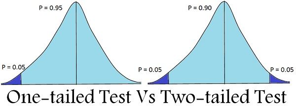
Multiply p by two to calculate the "*two-tailed p-value for the one-sample t statistic*".
```{r}
p * 2
```

If all went well, we should have gotten the same t and p value that R's built-in 
`t.test()` function would calculate.  Try it out below (and don't forget to set mu!).
How do your results compare?
```{r}
tstat <- t.test(deepsleep.before, mu = 180, alternative = 'two.sided')
tstat
```


## Goal 2: Repeated ("Paired") Samples T-test

   *Goal 2*: We want to conclude that the treatment *didn't do nothing* to the amount of deep sleep the patients obtained.
     (Yes, this is a funny way to describe the results. Such is hypothesis testing!)

Plot the two distributions of sleep amounts.  Do you think there's a difference?  What effect size do you expect in this comparison?     
```{r}

```

Luckily, this is a "repeated-sample" experiment; we measured the same people twice
and can simply subtract each person from each other.  Plot the distribution of these
differences.  What effect size do you expect now?
```{r}

```

Let's skip ahead to the R stage and just use the `t.test()` function.  Check the difference
in results between when you do an "independent-sample" t-test and a "paired-sample" ttest (setting different 
options).  Why do they give such different results?  What can we learn from each of these tests?
```{r}
t.test(deepsleep.after - deepsleep.before, mu=1)
```


Finally, let's write our report for these differences, including the t-values, the name of the test,
and the p-value.
"""
(write report here.)


"""



```{r}
library(pwr)
plot(pwr.t.test(n = NULL, d=0.5, sig.level = .001, power = .8, type='paired', alternative = 'greater'))
```



```{r}
dd <- data.frame(
  sleep=c(deepsleep.before, deepsleep.after), 
  group=c(rep("before", length(deepsleep.before)), rep("after", length(deepsleep.after)))
  # id=rep(seq(1, length(deepsleep.before)), 2)
)
dd
```