1.3-Model_validation_and_Resampling.qmd

---
title: "Model validation and Resampling"
author: "Alex Sanchez, Ferran Reverter and Esteban Vegas"
institute: "Genetics Microbiology and Statistics Department. University of Barcelona"
format:
  revealjs: 
    incremental: false  
    # transition: slide
    # background-transition: fade
    # transition-speed: slow
    scrollable: true
    menu:
      side: left
      width: half
      numbers: true
    slide-number: c/t
    show-slide-number: all
    progress: true
    css: "css4CU.css"
    theme: sky
    embed-resources: false
  beamer:
    aspectratio: 43
    navigation: horizontal
    # theme: AnnArbor
    # colortheme: lily
    theme: Frankfurt
    colortheme: default
    incremental: false
    slide-level: 2
    section-titles: false
    css: "css4CU.css"
    includes:
      in-header: "myheader.tex"  

#    suppress-bibliography: true
bibliography: "StatisticalLearning.bib"
editor_options: 
  chunk_output_type: console
editor: 
  markdown: 
    wrap: 72
---

# Model performance

## Assessing model performance

::: font80
-   Error estimation and, in general, performance assessment in
    predictive models is a complex process.

-   A key challenge is that *the true error of a model on new data is
    typically unknown*, and using the training error as a proxy leads to
    an optimistic evaluation.

-   Resampling methods, such as *cross-validation* and *the bootstrap*,
    allow us to approximate test error and assess model variability
    using only the available data.

-   What is best it can be proven that, well performed, they provide
    reliable estimates of a model’s performance.

-   This section introduces these techniques and discusses their
    practical implications in model assessment.
:::

## Prediction (generalization) error

-   We are interested the prediction or generalization error, the error
    that will appear when predicting a new observation using a model
    fitted from some dataset.

-   Although we don't know it, it can be estimated using either the
    training error or the test error estimators.

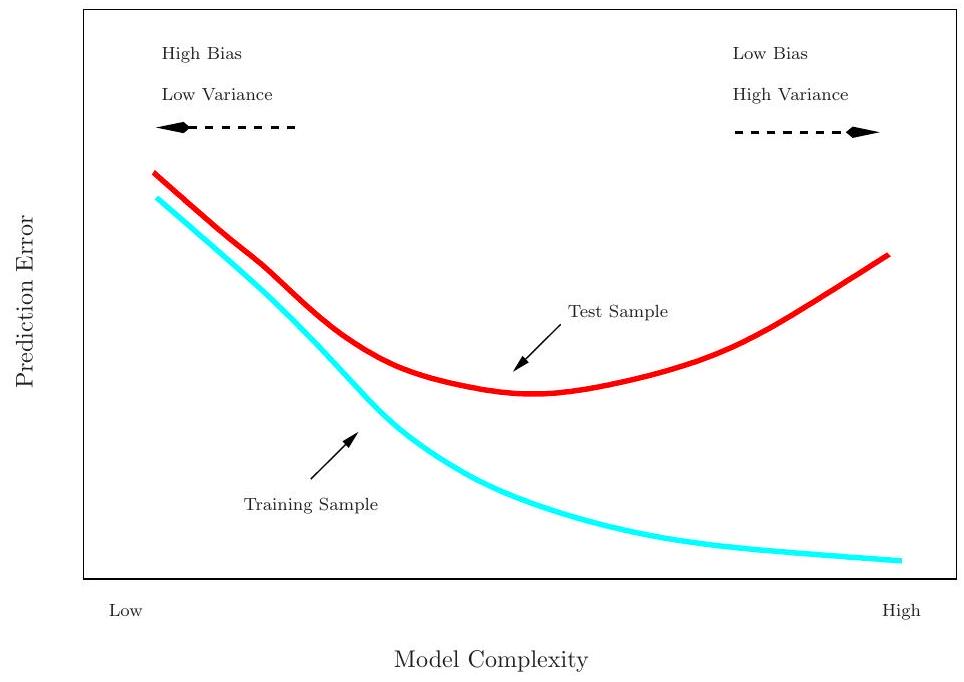
## Training Error vs Test error

-   The test error is the average error that results from using a
    statistical learning method to predict the response on a new
    observation, one that was not used in training the method.

-   The training error is calculated from the difference among the
    predictions of a model and the observations used to train it.

-   Training error rate often is quite different from the test error
    rate, and in particular the former can dramatically underestimate
    the latter.

## The three errors

::: font70

- **Generalization Error**. True expected test error (unknown). No bias  $$\mathcal{E}(f) =  \mathbb{E}_{X_0, Y_0} [ L(Y_0, f(X_0)) ]$$ 

- **Test Error Estimator**. Estimate of generalization error. Small bias. $$\hat{\mathcal{E}}_{\text{test}}=\frac{1}{m} \sum_{j=1}^{m} L(Y_j^{\text{test}},  f(X_j^{\text{test}}))$$ 

- **Training Error Estimator**. Measures fit to training data (optimistic). High bias $$\hat{\mathcal{E}}_{\text{train}}: \frac{1}{n} \sum_{i=1}^{n} L(Y_i^{\text{train}}, f(X_i^{\text{train}}))$$

:::

<!-- | Measure | Formula | Interpretation | Bias | -->
<!-- |---------------------------|---------------|---------------|---------------| -->
<!-- | **Generalization Error** $\mathcal{E}(f)$ | $\mathbb{E}_{X_0, Y_0} [ L(Y_0, f(X_0)) ]$ | True expected test error (unknown) | None | -->
<!-- | **Test Error Estimator** $\hat{\mathcal{E}}_{\text{test}}$ | $\frac{1}{m} \sum_{j=1}^{m} L(Y_j^{\text{test}}, f(X_j^{\text{test}}))$ | Estimate of generalization error (unbiased) | Low | -->
<!-- | **Training Error Estimator** $\hat{\mathcal{E}}_{\text{train}}$ | $\frac{1}{n} \sum_{i=1}^{n} L(Y_i^{\text{train}}, f(X_i^{\text{train}}))$ | Measures fit to training data (optimistic) | High | -->
<!-- ::: -->

## Training- versus Test-Set Performance

![](https://cdn.mathpix.com/cropped/2025_02_18_d84fddb1dda73076f5eag-05.jpg?height=682&width=964&top_left_y=157&top_left_x=151)

## Prediction-error estimates

-   Ideal: a large designated test set. Often not available

-   Some methods make a mathematical adjustment to the training error
    rate in order to estimate the test error rate: $Cp$ statistic, $AIC$
    and $BIC$.

-   Instead, we consider a class of methods that

    1.  Estimate test error by holding out a subset of the training
        observations from the fitting process, and
    2.  Apply learning method to held out observations

## Validation-set approach

-   Randomly divide the available samples into two parts: a *training
    set* and a *validation or hold-out set*.

-   The model is fit on the training set, and the fitted model is used
    to predict the responses for the observations *in the validation
    set*.

-   The resulting validation-set error provides an estimate of the test
    error. This is assessed using:

    -   MSE in the case of a quantitative response and
    -   Misclassification rate in qualitative response.

## The Validation process

![](https://cdn.mathpix.com/cropped/2025_02_18_d84fddb1dda73076f5eag-08.jpg?height=187&width=830&top_left_y=310&top_left_x=205)

A random splitting into two halves: left part is training set, right
part is validation set

## Example: automobile data

-   Goal: compare linear vs higher-order polynomial terms in a linear
    regression

-   Method: randomly split the 392 observations into two sets,

    -   Training set containing 196 of the data points,
    -   Validation set containing the remaining 196 observations.

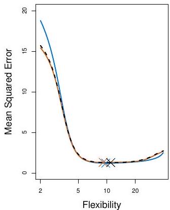
## Example: automobile data (plot)

![](https://cdn.mathpix.com/cropped/2025_02_18_d84fddb1dda73076f5eag-09.jpg?height=379&width=954&top_left_y=466&top_left_x=140)

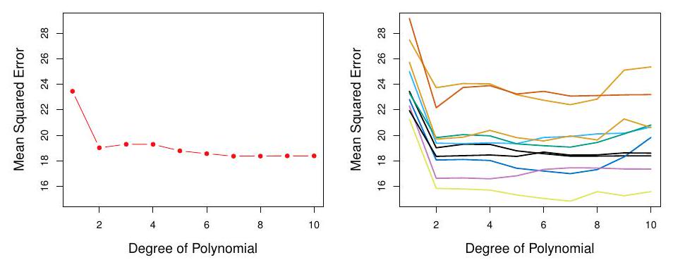
Left panel single split; Right panel shows multiple splits

## Drawbacks of the (VS) approach

::: font90
-   In the validation approach, *only a subset of the observations*
    -those that are included in the training set rather than in the
    validation set- are used to fit the model.

-   The validation estimate of the test error *can be highly variable*,
    depending on which observations are included in the training set and
    which are included in the validation set.

-   This suggests that *validation set error may tend to over-estimate
    the test error for the model fit on the entire data set*.
:::

# Cross-Validation

## $K$-fold Cross-validation

-   Widely used approach for estimating test error.

-   Estimates give an idea of the test error of the final chosen model

-   Estimates can be used to select best model,

## $K$-fold CV mechanism

-   Randomly divide the data into $K$ equal-sized parts.
-   Repeat for each part $k=1,2, \ldots K$,
    -   Leave one part, $k$, apart.
    -   Fit the model to the combined remaining $K-1$ parts,
    -   Then obtain predictions for the left-out $k$-th part.
-   Combine the results to obtain the crossvalidation estimate of tthe
    error.

## $K$-fold Cross-validation in detail

![](images/clipboard-2845603259.png){fig-align="center"}

::: font60
A schematic display of 5-fold CV. A set of n observations is randomly
split into fve non-overlapping groups. Each of these ffths acts as a
validation set (shown in beige), and the remainder as a training set
(shown in blue). The test error is estimated by averaging the fve
resulting MSE estimates
:::

## The details

::: font80
-   Let the $K$ parts be $C_{1}, C_{2}, \ldots C_{K}$, where $C_{k}$
    denotes the indices of the observations in part $k$. There are
    $n_{k}$ observations in part $k$ : if $N$ is a multiple of $K$, then
    $n_{k}=n / K$.

-   Compute $$
    \mathrm{CV}_{(K)}=\sum_{k=1}^{K} \frac{n_{k}}{n} \mathrm{MSE}_{k}
    $$ where
    $\mathrm{MSE}_{k}=\sum_{i \in C_{k}}\left(y_{i}-\hat{y}_{i}\right)^{2} / n_{k}$,
    and $\hat{y}_{i}$ is the fit for observation $i$, obtained from the
    data with part $k$ removed.

-   $K=n$ yields $n$-fold or *leave-one out cross-validation (LOOCV)*.
:::

<!-- ## A nice special case! -->

<!-- -   With least-squares linear or polynomial regression, an amazing shortcut makes the cost of LOOCV the same as that of a single model -->

<!--     fit! The following formula holds: -->

<!-- $$ -->

<!-- \mathrm{CV}_{(n)}=\frac{1}{n} \sum_{i=1}^{n}\left(\frac{y_{i}-\hat{y}_{i}}{1-h_{i}}\right)^{2} -->

<!-- $$ -->

<!-- where $\hat{y}_{i}$ is the $i$ th fitted value from the original least -->

<!-- squares fit, and $h_{i}$ is the leverage (diagonal of the "hat" matrix; -->

<!-- see book for details.) This is like the ordinary MSE, except the $i$ th -->

<!-- residual is divided by $1-h_{i}$. -->

<!-- -   LOOCV sometimes useful, but typically doesn't shake up the data -->

<!--     enough. The estimates from each fold are highly correlated and hence -->

<!--     their average can have high variance. -->

<!-- -   a better choice is $K=5$ or 10 . -->

## Auto data revisited

![](images/clipboard-3294277508.png)

<!-- ## True and estimated test MSE for the simulated data -->

<!-- ![](https://cdn.mathpix.com/cropped/2025_02_18_d84fddb1dda73076f5eag-19.jpg?height=419&width=348&top_left_y=292&top_left_x=90) -->
<!-- ![](https://cdn.mathpix.com/cropped/2025_02_18_d84fddb1dda73076f5eag-19.jpg?height=415&width=339&top_left_y=294&top_left_x=446) -->
<!-- ![](https://cdn.mathpix.com/cropped/2025_02_18_d84fddb1dda73076f5eag-19.jpg?height=414&width=335&top_left_y=293&top_left_x=803) -->

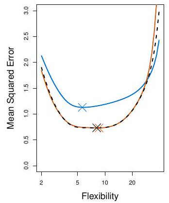
## Issues with Cross-validation

-   Since each training set is only $(K-1) / K$ as big as the original training set, the estimates of prediction error will typically be biased upward. Why?
-   This bias is minimized when $K=n$ (LOOCV), but this estimate has high variance, as noted earlier.
-   $K=5$ or 10 provides a good compromise for this bias-variance
    tradeoff.

## CV for Classification Problems

::: font80

-   Divide the data into $K$ roughly equal-sized parts $C_{1}, C_{2}, \ldots C_{K}$.

<!-- $C_{k}$ denotes the indices of the observations in part $k$.  -->

- There are $n_{k}$ observations in part $k$
and $n_{k}\simeq n / K$.
-   Compute
$$
\mathrm{CV}_{K}=\sum_{k=1}^{K} \frac{n_{k}}{n} \operatorname{Err}_{k}
$$
where
$\operatorname{Err}_{k}=\sum_{i \in C_{k}} I\left(y_{i} \neq \hat{y}_{i}\right) / n_{k}$.

:::

## Standard error of CV estimate

-   The estimated standard deviation of $\mathrm{CV}_{K}$ is:

$$
\widehat{\mathrm{SE}}\left(\mathrm{CV}_{K}\right)=\sqrt{\frac{1}{K} \sum_{k=1}^{K} \frac{\left(\operatorname{Err}_{k}-\overline{\operatorname{Err}_{k}}\right)^{2}}{K-1}}
$$

-   This is a useful estimate, but strictly speaking, not quite valid. Why not?

## Why is this an issue?

::: font80

- In \(K\)-fold CV, the same dataset is used repeatedly for training and testing across different folds. 
- This introduces **correlations** between  estimated errors in different folds because each fold's training set overlaps  with others.

- The assumption underlying this estimation of the standard error is that $\operatorname{Err}_{k}$ values are **independent**, which does not hold here.
- The dependence between folds leads to **underestimation** of the true variability in $\mathrm{CV}_K$, meaning that the reported standard error is likely **too small**, giving a misleading sense of precision in the estimate of the test error.

:::

## CV: right and wrong

<!-- - CV needs to be performed the right way beacause it is easy to misunderstand how to do it well. -->

- Consider a classifier applied to some 2-class data:

  1.  Start with 5000 predictors & 50 samples and find the 100 predictors most correlated with the class labels.
  2.  We then apply a classifier such as logistic regression, using only these 100 predictors.

- In order to estimate the test set performance of this classifier, _¿can we apply cross-validation in step 2, forgetting about step 1?_

## CV the Wrong and the Right way

::: font90

-   Applying CV only to Step 2 ignores the fact that in Step 1, the procedure has already used the labels of the training data.

  - This is a form of training and **must be included in the validation process**.

    - Wrong way: Apply cross-validation in step 2.
    - Right way: Apply cross-validation to steps 1 and 2.

-   This error has happened in many high profile papers, mainly due to a misunderstanding of what CV means and does.

:::


## Wrong Way

![](https://cdn.mathpix.com/cropped/2025_02_18_d84fddb1dda73076f5eag-31.jpg?height=503&width=1068&top_left_y=229&top_left_x=101)

## Right Way

![](https://cdn.mathpix.com/cropped/2025_02_18_d84fddb1dda73076f5eag-32.jpg?height=499&width=1036&top_left_y=234&top_left_x=112)

# The Bootstrap

## Introducing the *Bootstrap*

-   A flexible and powerful statistical tool that can be used to quantify the uncertainty associated with an estimator or a statistical learning method.

- It can provide estimates of the standard error or confidence intervals for that estimator/method.

- Indeed, it can be applied to any (or most) situations where one needs to deal with variability, that the method can approximate using *resampling*.


## Where does the name came from?

-   The term derives from the phrase "to pull oneself up by one's bootstraps",  thought to be based on the XVIIIth century book " _The Surprising Adventures of Baron Munchausen_".

-   It is not the same as the term "bootstrap" used in computer science
    meaning to "boot" a computer from a set of core instructions.
    
## Origins of the bootstrap

:::: {.columns}

::: {.column width='60%'}

```{r}
knitr::include_graphics("images/Efron_y_Hastie.png")
```

:::

::: {.column width='40%'}

```{r}
knitr::include_graphics("images/bootLluisCasals.png")
```

:::

::::


## A simple example

-   Suppose that we wish to invest a fixed sum of money in two financial
    assets that yield returns of $X$ and $Y$, respectively, where $X$
    and $Y$ are random quantities.
-   We will invest a fraction $\alpha$ of our money in $X$, and will
    invest the remaining $1-\alpha$ in $Y$.
-   We wish to choose $\alpha$ to minimize the total risk, or variance,
    of our investment. In other words, we want to minimize
    $\operatorname{Var}(\alpha X+(1-\alpha) Y)$.

## Example continued

-   The value that minimizes the risk is: 
$$
\alpha=\frac{\sigma_{Y}^{2}-\sigma_{X Y}}{\sigma_{X}^{2}+\sigma_{Y}^{2}-2 \sigma_{X Y}}
$$
where: 

    - $\sigma_{X}^{2}=\operatorname{Var}(X)$
     - $\sigma_{Y}^{2}=\operatorname{Var}(Y)$ and
     
    - $\sigma_{X Y}=\operatorname{Cov}(X, Y)$.

## Example continued

-   The values of $\sigma_{X}^{2}, \sigma_{Y}^{2}$, and $\sigma_{X Y}$ are unknown.
-   We can compute estimates for these quantities,
    $\hat{\sigma}_{X}^{2}, \hat{\sigma}_{Y}^{2}$, and
    $\hat{\sigma}_{X Y}$, using a data set that contains measurements
    for $X$ and $Y$.
-   We can then estimate the value of $\alpha$ that minimizes the
    variance of our investment using
$$
\hat{\alpha}=\frac{\hat{\sigma}_{Y}^{2}-\hat{\sigma}_{X Y}}{\hat{\sigma}_{X}^{2}+\hat{\sigma}_{Y}^{2}-2 \hat{\sigma}_{X Y}}
$$

## Example continued

```{r, out.width="100%", fig.cap='Each panel displays 100 simulated returns for investments $X$ and $Y$. <br> From left to right and top to bottom, the resulting estimates for alpha are<br> 0.576, 0.532, 0.657, and 0.651'}
knitr::include_graphics("images/bootExample1.png")
```



## Example: How variable is $\hat \alpha$?

::: font90

- The standard deviation of $\hat{\alpha}$, can be estimated as:

  - 1. Repeat 1 ... 1000 times
  
    -  1.1 Simulate 100 paired observations of $X$ and $Y$.
    - 1.2 Estimate $\alpha: \hat{\alpha}_{1}, \hat{\alpha}_{2}, \ldots, \hat{\alpha}_{1000}$.
  
  - 2. Compute the standard deviation of $\alpha_i$, $s_{1000}(\hat{\alpha}_i)$ and use it as an estimator of $SE (\hat{\alpha})$
  
  - 3. The sample mean of all $\alpha_i$, $\overline{\hat{\alpha}_i}$ is also a monte carlo estimate of $\alpha$, although we are not interested in it.

:::

## Example: Simlation results

```{r out.width="90%"}
knitr::include_graphics("images/simulatedAlfaValues.png")
```

::: font50

Left: A histogram of the estimates of $\alpha$ obtained by generating 1,000 simulated data sets from the true population. Center: A histogram of the estimates of $\alpha$ obtained from 1,000 bootstrap
samples from a single data set. Right: The estimates of $\alpha$ displayed in the left and center panels are shown as boxplots. 

For these simulations the parameters were set to  $\sigma_{X}^{2}=1, \sigma_{Y}^{2}=1.25$, and $\sigma_{X Y}=0.5$, and  so we know that the true value of $\alpha$ is 0.6 (indicated by the red line).
:::

## Example continued

::: font70

-   The mean over all 1,000 estimates for $\alpha$ is

$$
\bar{\alpha}=\frac{1}{1000} \sum_{r=1}^{1000} \hat{\alpha}_{r}=0.5996,\quad \text { very close to $\alpha=0.6$.}
$$

- The standard deviation of the estimates computed on the simulated samples:
$$
\mathrm{SE}_{Sim}(\hat{\alpha})= \sqrt{\frac{1}{1000-1} \sum_{r=1}^{1000}\left(\hat{\alpha}_{r}-\bar{\alpha}\right)^{2}}=0.083
$$

-   This gives an idea of the accuracy of $\hat{\alpha}$ :
    $\mathrm{SE}(\hat{\alpha}) \approx \mathrm{SE}_{Sim}(\hat{\alpha})= 0.083$.
-   So roughly speaking, for a random sample from the population, we
    would expect $\hat{\alpha}$ to differ from $\alpha$ by approximately
    0.08 , on average.

:::

## Back to the real world

-   The procedure outlined above, Monte Carlo Sampling,  cannot be applied, because *for real data we cannot generate new samples from the original population*.

-   However, the bootstrap approach allows us to use a computer to mimic  the process of obtaining new data sets, so that we can estimate the variability of our estimate without generating additional samples.

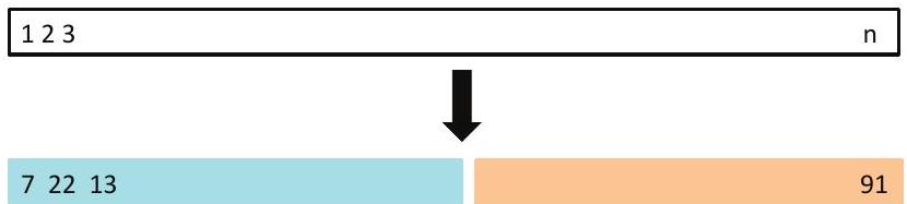
## Sampling the sample = *resampling*
-   Rather than repeatedly obtaining independent data sets from the population, we may obtain distinct data sets by *repeatedly sampling observations from the original data set with replacement*.

-   This generates a list of "bootstrap data sets" of the same size as our original dataset. 

- As a result some observations may appear more than once in a given  bootstrap data set and some not at all.



## Resampling illustrated

```{r, fig.align='center', out.width="100%"}
knitr::include_graphics("images/1.2-Ensemble_Methods-Slides_insertimage_2.png")
```

## Boot. estimate of std error {.smaller}

- The standard error of $\alpha$ can be approximated by the the standard deviation taken on all of these bootstrap estimates using  the usual formula:
$$
\mathrm{SE}_{B}(\hat{\alpha})=\sqrt{\frac{1}{B-1} \sum_{r=1}^{B}\left(\hat{\alpha}^{* r}-\overline{\hat{\alpha^{*}}}\right)^{2}}
$$

-   This quantity, called *bootstrap estimate of standard error*  serves as an estimate of the standard error of $\hat{\alpha}$  estimated from the original data set. 
$$
\mathrm{SE}_{B}(\hat{\alpha}) \approx \mathrm{SE}(\hat{\alpha})
$$

- For this example $\mathrm{SE}_{B}(\hat{\alpha})=0.087$.

## A general picture for the bootstrap

![](https://cdn.mathpix.com/cropped/2025_02_18_d84fddb1dda73076f5eag-45.jpg?height=456&width=1072&top_left_y=248&top_left_x=98)

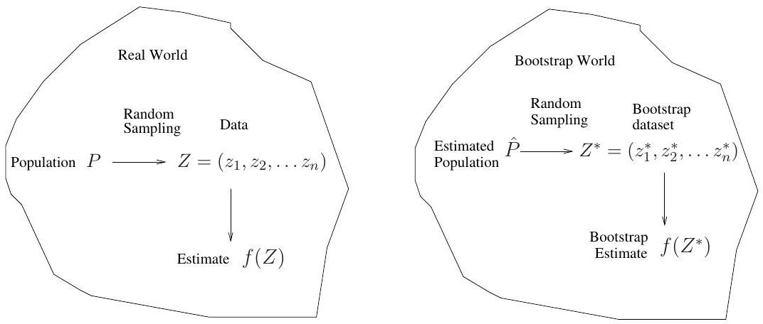
## The bootstrap in general

-   In more complex data situations, figuring out the appropriate way to
    generate bootstrap samples can require some thought.
-   For example, if the data is a time series, we can't simply sample
    the observations with replacement (why not?).
-   We can instead create blocks of consecutive observations, and sample
    those with replacements. Then we paste together sampled blocks to
    obtain a bootstrap dataset.

## Other uses of the bootstrap

-   Primarily used to obtain standard errors of an estimate.
-   Also provides approximate confidence intervals for a population
    parameter. For example, looking at the histogram in the middle panel
    of the Figure on slide 29, the $5 \%$ and $95 \%$ quantiles of the
    1000 values is (.43, .72 ).
-   This represents an approximate $90 \%$ confidence interval for the
    true $\alpha$. How do we interpret this confidence interval?

## Other uses of the bootstrap

-   Primarily used to obtain standard errors of an estimate.

-   Also provides approximate confidence intervals for a population
    parameter. For example, looking at the histogram in the middle panel
    of the Figure on slide 29, the $5 \%$ and $95 \%$ quantiles of the
    1000 values is (.43, .72 ).

-   This represents an approximate $90 \%$ confidence interval for the
    true $\alpha$. How do we interpret this confidence interval?

-   The above interval is called a Bootstrap Percentile confidence
    interval. It is the simplest method (among many approaches) for
    obtaining a confidence interval from the bootstrap.

## Can the bootstrap estimate prediction error?

-   In cross-validation, each of the $K$ validation folds is distinct
    from the other $K-1$ folds used for training: there is no overlap.
    This is crucial for its success. Why?

-   To estimate prediction error using the bootstrap, we could think
    about using each bootstrap dataset as our training sample, and the
    original sample as our validation sample.

-   But each bootstrap sample has significant overlap with the original
    data. About two-thirds of the original data points appear in each
    bootstrap sample. Can you prove this?

-   This will cause the bootstrap to seriously underestimate the true
    prediction error. Why?

-   The other way around- with original sample = training sample,
    bootstrap dataset $=$ validation sample - is worse!

## Removing the overlap

-   Can partly fix this problem by only using predictions for those
    observations that did not (by chance) occur in the current bootstrap
    sample.

-   But the method gets complicated, and in the end, cross-validation
    provides a simpler, more attractive approach for estimating
    prediction error.

## Pre-validation

-   In microarray and other genomic studies, an important problem is to
    compare a predictor of disease outcome derived from a large number
    of "biomarkers" to standard clinical predictors.

-   Comparing them on the same dataset that was used to derive the
    biomarker predictor can lead to results strongly biased in favor of
    the biomarker predictor.

-   Pre-validation can be used to make a fairer comparison between the
    two sets of predictors.

## Motivating example

An example of this problem arose in the paper of van't Veer et al.
Nature (2002). Their microarray data has 4918 genes measured over 78
cases, taken from a study of breast cancer. There are 44 cases in the
good prognosis group and 34 in the poor prognosis group. A "microarray"
predictor was constructed as follows:

1.  70 genes were selected, having largest absolute correlation with the
    78 class labels.
2.  Using these 70 genes, a nearest-centroid classifier $C(x)$ was
    constructed.
3.  Applying the classifier to the 78 microarrays gave a dichotomous
    predictor $z_{i}=C\left(x_{i}\right)$ for each case $i$.

## Results

Comparison of the microarray predictor with some clinical predictors,
using logistic regression with outcome prognosis:

| Model      |          Coef | Stand. Err. | Z score | p-value |
|:-----------|--------------:|------------:|--------:|--------:|
| Re-use     |               |             |         |         |
| microarray |         4.096 |       1.092 |   3.753 |   0.000 |
| angio      |         1.208 |       0.816 |   1.482 |   0.069 |
| er         |        -0.554 |       1.044 |  -0.530 |   0.298 |
| grade      |        -0.697 |       1.003 |  -0.695 |   0.243 |
| pr         |         1.214 |       1.057 |   1.149 |   0.125 |
| age        |        -1.593 |       0.911 |  -1.748 |   0.040 |
| size       |         1.483 |       0.732 |   2.026 |   0.021 |
|            | Pre-validated |             |         |         |
|            |               |             |         |         |
| microarray |         1.549 |       0.675 |   2.296 |   0.011 |
| angio      |         1.589 |       0.682 |   2.329 |   0.010 |
| er         |        -0.617 |       0.894 |  -0.690 |   0.245 |
| grade      |         0.719 |       0.720 |   0.999 |   0.159 |
| pr         |         0.537 |       0.863 |   0.622 |   0.267 |
| age        |        -1.471 |       0.701 |  -2.099 |   0.018 |
| size       |         0.998 |       0.594 |   1.681 |   0.046 |

## Idea behind Pre-validation

-   Designed for comparison of adaptively derived predictors to fixed,
    pre-defined predictors.

-   The idea is to form a "pre-validated" version of the adaptive
    predictor: specifically, a "fairer" version that hasn't "seen" the
    response $y$.

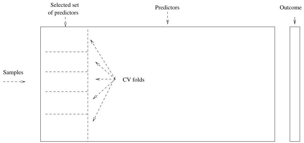
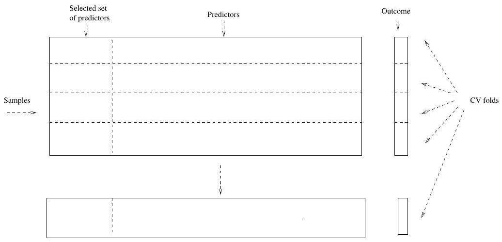
## Pre-validation process

![](https://cdn.mathpix.com/cropped/2025_02_18_d84fddb1dda73076f5eag-64.jpg?height=760&width=812&top_left_y=139&top_left_x=229)

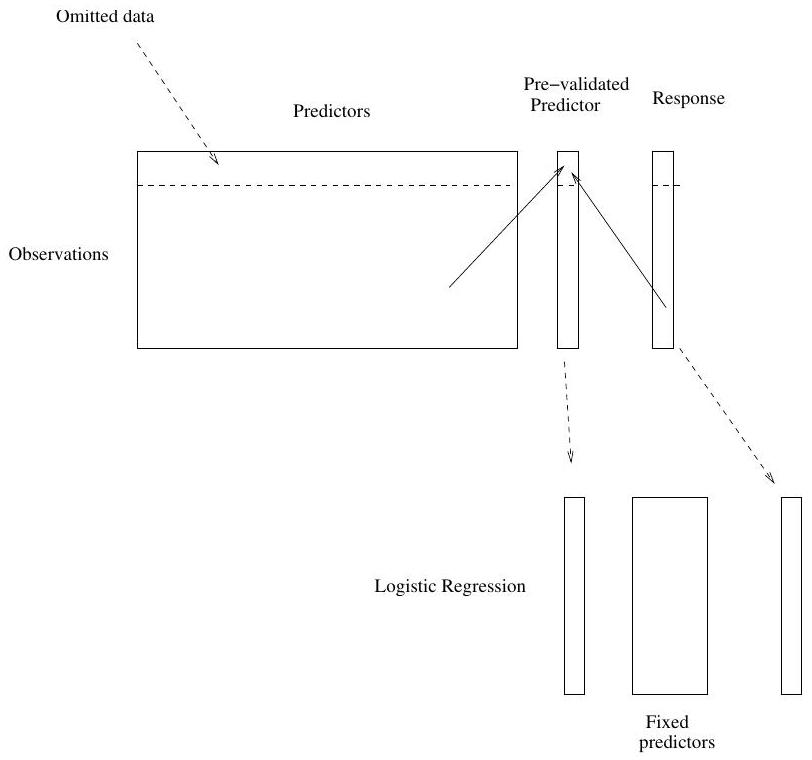
## Pre-validation in detail for this example

1.  Divide the cases up into $K=13$ equal-sized parts of 6 cases each.
2.  Set aside one of parts. Using only the data from the other 12 parts,
    select the features having absolute correlation at least .3 with the
    class labels, and form a nearest centroid classification rule.
3.  Use the rule to predict the class labels for the 13th part
4.  Do steps 2 and 3 for each of the 13 parts, yielding a
    "pre-validated" microarray predictor $\tilde{z}_{i}$ for each of the
    78 cases.
5.  Fit a logistic regression model to the pre-validated microarray
    predictor and the 6 clinical predictors.

## The Bootstrap versus Permutation tests

-   The bootstrap samples from the estimated population, and uses the
    results to estimate standard errors and confidence intervals.

-   Permutation methods sample from an estimated null distribution for
    the data, and use this to estimate p-values and False Discovery
    Rates for hypothesis tests.

-   The bootstrap can be used to test a null hypothesis in simple
    situations. Eg if $\theta=0$ is the null hypothesis, we check
    whether the confidence interval for $\theta$ contains zero.

-   Can also adapt the bootstrap to sample from a null distribution (See
    Efron and Tibshirani book "An Introduction to the Bootstrap" (1993),
    chapter 16) but there's no real advantage over permutations.